Glossary page M
Margin of error
A number used to give an indication of the amount of uncertainty due to sampling error when using data from a random sample to estimate a population parameter.
The margin of error is often used in media reports of survey results. Many of these reports state estimates (sample proportions) of population proportions along with a margin of error. The margin of error is a mathematical calculation based on a confidence level of 95% for confidence intervals for each population proportion. In fact the margin of error for a sample proportion varies as the proportion varies but the stated margin of error is the largest of these possible margins of error.
An approximate 95% confidence interval for a population proportion or a difference between population proportions can be formed by:
- subtracting the margin of error from the estimate to obtain the lower limit, and
- adding the margin of error to the estimate to obtain the upper limit.

If you cannot view or read this diagram/graph, select this link to
open a text version.
Note: For any given survey or sample, the largest possible margin of error is determined by the sample size.
At Level 8 some “rules of thumb” for estimating and using margins of error are suggested.
 Rule of Thumb
For poll percentages between 30% and 70% the margin of error ≈
 , where n is the sample size.
For poll percentages below 30% and above 70% the margin of error is smaller
than
 .
.
See Example 2 below.
2 x Margin of Error Rule of Thumb (Comparisons within one group)
For two different responses within the same group, the margin of error for the difference between two proportions is 2 times the margin of error for that poll or group.
See Example 3 below.
1.5 x Average Margin of Error Rule of Thumb (Comparisons between two independent groups)
For responses from two independent groups, the margin of error for the difference between the two proportions is 1.5 times the average of the margins of error for the two polls or groups.
See Example 4 below.
Example 1
In a poll of 1000 randomly selected eligible New Zealand voters taken in May 2013, 47.1% of respondents stated they would give their party vote to the National party. The polling agency stated that the poll had a maximum margin of error of 3.2%.
47.1 – 3.2 = 43.9 and 47.1 + 3.2 = 50.3
Based on this survey data, an approximate 95% confidence interval for the percentage support for the National party for all eligible voters is 43.9%, 50.3%.
Example 2
In a poll of 1000 randomly selected eligible New Zealand voters taken in July 2013, about 41% of respondents chose John Key as their preferred Prime Minister.
Using the
 rule of thumb the approximate margin of error is

Example 3
In a poll of 1000 randomly selected eligible New Zealand voters taken in May 2013, 47.1% of respondents stated they would give their party vote to the National party and 33.1% would give their party vote to the Labour party. The polling agency stated that the poll had a maximum margin of error of 3.2%. Does this allow a claim to be made that, for all New Zealand voters, National is ahead of Labour in the party vote?
- Difference in poll percentages
- = 47.1 - 33.1
- = 14.0 percentage points
- 2 x margin of error
- = 2 x 3.2
- = 6.4 percentage points
Approximate 95% confidence interval for difference in proportions:
- Lower limit
- = 14.0 - 6.4
- = 7.6 percentage points
- Upper limit
- = 14.0 + 6.4
- = 20.4 percentage points
An approximate 95% confidence interval is (7.6 percentage points, 20.4 percentage points).
With 95% confidence, we estimate that taken over all New Zealand voters support for the National party is somewhere between 7.6 and 20.4 percentage points higher than that for the Labour Party. It can be claimed that, for all New Zealand voters, National is ahead of Labour in the party vote.
Example 4
In a poll, randomly selected New Zealanders over the age of 15 were asked about the impact the economy is having on their financial situation. Of the 225 respondents aged 30 to 49, 72 (55.8%) replied that it had had a big impact. Of the 248 respondents aged 50 and over, 42 (32.6%) replied that it had had a big impact. Does this allow a claim to be made that the percentage of 30 to 49 year old New Zealanders who think the economy is having a big impact on their financial situation is greater than the corresponding percentage of New Zealanders aged 50 and over?
- Difference in poll percentages
- = 55.8 - 32.6
- = 23.2 percentage points
Margin of error for 30 to 49 group ≈

Margin of error for 50 and over group ≈

Average margin of error = 6.55%
- 1.5 x average margin of error
Approximate 95% confidence interval for difference in proportions:
- Lower limit = 23.2 – 9.825
- Upper limit = 23.2 + 9.825
An approximate 95% confidence interval is (13.4 percentage points, 33.0 percentage points).
With 95% confidence, we estimate that the percentage of 30 to 49 year old New Zealanders who think the economy is having a big impact on their financial situation is somewhere between 13.4 and 33.0 percentage points greater than the corresponding percentage of New Zealanders aged 50 and over. It can be claimed that the percentage of 30 to 49 year old New Zealanders who think the economy is having a big impact on their financial situation is greater than the corresponding percentage of New Zealanders aged 50 and over.
See: sampling error
Curriculum achievement objectives references
Statistical literacy: Level 8
Mean
A measure of centre for a distribution of a numerical variable. The mean is the centre of mass of the values in a distribution and is calculated by adding the values and then dividing this total by the number of values.
For large data sets, it is recommended that a calculator or software is used to calculate the mean.
The mean can be influenced by unusually large or unusually small values. It is recommended that a graph of the distribution is used to check the appropriateness of the mean as a measure of centre and to emphasise its meaning as a feature of the distribution.
Example
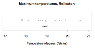
The maximum temperatures, in degrees Celsius (°C), in Rolleston for the first 10 days in November 2008 were 18.6, 19.9, 20.6, 19.4, 17.8, 18.1, 17.8, 18.7, 19.6, 18.8
The mean maximum temperature over these 10 days was 18.93°C.
The data and the mean are displayed on the dot plot below.

If you cannot view or read this graph, select this link to
open a text version.
Alternative: arithmetic mean
See: measure of centre, population mean, sample mean
Curriculum achievement objectives references
Statistical investigation: Levels 5, (6), (7), 8
Measure
An amount or quantity that is determined by measurement or calculation. The term ‘measure’ is used in two different ways in the curriculum.
One use is in the terms measure of centre, measure of spread, and measure of proportion, where these measures are calculated quantities that represent characteristics of a distribution. The use of ‘using displays and measures’ in the level 6 (statistical investigation thread) achievement objective is a reference to measures of centre, spread, and proportion.
The other use applies to a statistical investigation. The investigator decides on a subject of interest and then decides the aspects of it that can be observed. These aspects are the ‘measures’.
Example
An investigator decides that ‘well-being’ is a subject of interest and chooses ‘happiness’ to be one aspect of well-being. Happiness could be measured by the variable ‘the average number of times a person laughs in a day’.
Curriculum achievement objectives references
Statistical investigation: Levels 5, 6, 7, (8)
Statistical literacy: Levels 5, (6), (7), (8)
Measure of centre
A number that is representative or typical of the middle of a distribution of a numerical variable. The measures of centre that are used most often are the mean and the median. The mode is sometimes used.
Alternatives: measure of centrality, measure of central tendency, measure of location
See: average
Curriculum achievement objectives references
Statistical investigation: Levels 5, (6), (7), (8)
Measure of proportion
A sample proportion used to make comparisons among sample distributions.
Example
An online questionnaire was completed by 727 students enrolled in an introductory statistics course at the University of Auckland. It included questions on their actual weight, gender, and ethnicity.
The measurement variable ‘actual weight’ was recategorised with one category for actual weights less than 60 kg. It was concluded that 56.7% of the females weighed less than 60 kg compared with 7.6% of the males. This is an example of bivariate data with one measurement variable (actual weight) and one category variable (gender).
As part of a comparison between the ethnicity sample distributions for females and males, it was concluded that 5.4% of the females were Korean compared with 10.9% of the males. This is an example of bivariate data with two category variables.
Curriculum achievement objectives references
Statistical investigation: Levels 5, (6), (7), (8)
Measure of spread
A number that conveys the degree to which values in a distribution of a numerical variable differ from each other. The measures of spread that are used most often are interquartile range, range, standard deviation, and variance.
Alternatives: measure of variability, measure of dispersion
Curriculum achievement objectives references
Statistical investigation: Levels 5, (6), (7), (8)
Measurement data
Data in which the values result from measuring, meaning that the values may take on any value within an interval of numbers.
Example
The heights of a class of year 9 students.
See: numerical data, quantitative data
Curriculum achievement objectives references
Statistical investigation: Level 4, (5), (6), (7), (8)
Measurement variable
A property that may have different values for different individuals and for which these values result from measuring, meaning that the values may take on any value within an interval of numbers.
Example
The heights of a class of year 9 students.
See: numerical variable, quantitative variable
Curriculum achievement objectives references
Statistical investigation: Levels (4), (5), (6), (7), (8)
Median
A measure of centre that marks the middle of a distribution of a numerical variable.
It is recommended that, for small data sets, this measure of centre is calculated by sorting the values into order and then counting the values, using software for large data sets.
The median is a stable measure of centre in that it is not influenced by unusually large or unusually small values. It is recommended that a graph of the distribution is used to emphasise its meaning as a feature of the distribution.
Example 1 (odd number of values)
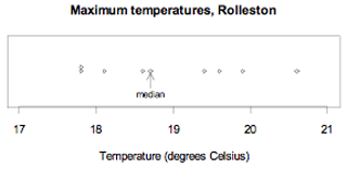
The maximum temperatures, in degrees Celsius (°C), in Rolleston for the first 9 days in November 2008 were 18.6, 19.9, 20.6, 19.4, 17.8, 18.1, 17.8, 18.7, 19.6
Ordered values: 17.8, 17.8, 18.1, 18.6, 18.7, 19.4, 19.6, 19.9, 20.6
The data and the median are displayed on the dot plot below.

If you cannot view or read this graph, select this link to
open a text version.
The median maximum temperature over these 9 days is 18.7°C. There are 4 values below 18.7°C and 4 values above it.
Example 2 (even number of values)
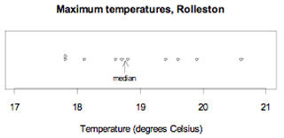
The maximum temperatures, in degrees Celsius (°C), in Rolleston for the first 10 days in November 2008 were 18.6, 19.9, 20.6, 19.4, 17.8, 18.1, 17.8, 18.7, 19.6, 18.8
Ordered values: 17.8, 17.8, 18.1, 18.6, 18.7, 18.8, 19.4, 19.6, 19.9, 20.6
The mean of the two central values, 18.7 and 18.8, is 18.75.
The data and the median are displayed on the dot plot below.

If you cannot view or read this graph, select this link to
open a text version.
The median maximum temperature over these 10 days is 18.75°C. There are 5 values below 18.75°C and 5 values above it.
Note: The median can be calculated directly from the dot plot or from the ordered values.
See: measure of centre
Curriculum achievement objectives references
Statistical investigation: Levels (5), (6), (7), (8)
Modal interval
An interval of neighbouring values for a measurement variable that occur noticeably more often than the values on each side of this interval.
Example
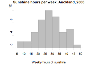
The number of hours of sunshine per week in Grey Lynn, Auckland, from Monday 2 January 2006 to Sunday 31 December 2006 is displayed in the histogram below.

If you cannot view or read this graph, select this link to
open a text version.
The distribution has a modal interval of 25 to 30 hours of sunshine per week.
Curriculum achievement objectives references
Statistical investigation: Levels (4), (5), (6), (7), (8)
Modality
A measure of the number of modes in a distribution of a numerical variable.
A unimodal distribution has one mode, meaning that the distribution has one value (or interval of neighbouring values) that occurs noticeably more often than any other value (or values on each side of the modal interval).
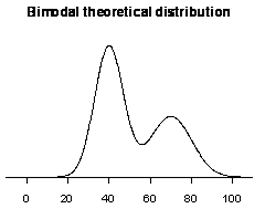
A bimodal distribution has two modes, meaning that the distribution has two values (or intervals of neighbouring values) that occur noticeably more often than the values on each side of the modes (or modal intervals).
In frequency distributions of a numerical variable the word cluster is often used to describe groups of neighbouring values that form modes or modal intervals.
Example 1 (frequency distribution, whole-number variable)
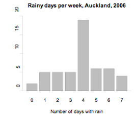
The number of days in a week that rain fell in Grey Lynn, Auckland, from Monday 2 January 2006 to Sunday 31 December 2006 is recorded in the frequency table and displayed in the bar graph below.
Count of weeks by number of days with rain – unimodal
| 0
| 2
|
| 1
| 5
|
| 2
| 5
|
| 3
| 5
|
| 4
| 19
|
| 5
| 6
|
| 6
| 6
|
| 7
| 4
|
| Total
| 52
|

If you cannot view or read this graph, select this link to
open a text version.
This distribution is unimodal with a mode at 4 days of rain per week.
Example 2 (theoretical distribution, continuous random variable)

The graph displays the probability density function of a theoretical distribution. It has modes at 40 and 70.
Curriculum achievement objectives references
Statistical investigation: Levels (6), (7), (8)
Mode
A value in a distribution of a numerical variable that occurs more frequently than other values.
As a measure of centre the mode is less useful than the mean or median because some distributions have more than one mode and other distributions, where no values are repeated, have no mode.
It is recommended that a graph of the distribution is used to check the appropriateness of the mode as a measure of centre and to emphasise its meaning as a feature of the distribution.
Example
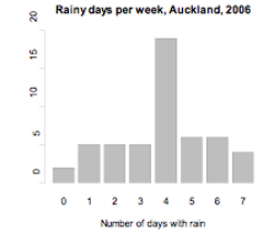
The number of days in a week that rain fell in Grey Lynn, Auckland, from Monday 2 January 2006 to Sunday 31 December 2006 is recorded in the frequency table and displayed on the bar graph below.
Count of weeks by number of days with rain – mode of 4 days
| 0
| 2
|
| 1
| 5
|
| 2
| 5
|
| 3
| 5
|
| 4
| 19
|
| 5
| 6
|
| 6
| 6
|
| 7
| 4
|
| Total
| 52
|

If you cannot view or read this graph, select this link to
open a text version.
The mode is 4 days with rain per week.
Curriculum achievement objectives references
Statistical investigation: Levels (5), (6), (7), (8)
Model
A simplified or idealised description of a situation. Model is used in two different ways in the curriculum.
In the probability thread, the use of ‘models of all the outcomes’ refers to a list of all possible outcomes of a situation involving elements of chance and, at more advanced levels, a list of all possible outcomes and the corresponding probabilities for each outcome.
At level 8 in the statistical investigation thread, an achievement objective refers to ‘appropriate models (including linear regression for bivariate data and additive models for time-series data)’. Used in this way, a model is an idealised description of the underlying system the data was taken from, and the model is intended to match the data closely.
See: probability function (for a discrete random variable)
Curriculum achievement objectives references
Statistical investigation: Level 8
Probability: Levels 3, 4, (5), (6), (7), (8)
Moving average
A method used to smooth time-series data. It forms a new smoothed series in which the irregular component is reduced.
If the time series has a seasonal component, a moving average is used to eliminate the seasonal component.
Each value in the time series is replaced by an average of the value and a number of neighbouring values. The number of values used to calculate a moving average depends on the type of time-series data. For weekly data, seven values are used; for monthly data, 12 values are used, and for quarterly data, four values are used. If the number of values used is even, the moving average must be centred by taking a two-term moving average of the new series.
In terms of an additive model for time-series data, Y = T + S + C + I, where
T represents the trend component,
S represents the seasonal component,
C represents the cyclical component, and
I represents the irregular component;
the smoothed series = T + C.
See: centred moving average, moving mean
Curriculum achievement objectives reference
Statistical investigation: Level (8)
Moving mean
A specified moving average method used to smooth time-series data. It forms a new smoothed series in which the irregular component is reduced.
If the time series has a seasonal component, a moving mean may be used to eliminate the seasonal component.
Each value in the time series is replaced by the mean of the value and a number of neighbouring values. The number of values used to calculate a moving mean depends on the type of time-series data. For weekly data, seven values are used, for monthly data, 12 values are used, and for quarterly data, four values are used. If the number of values used is even, the moving mean must be centred by taking two-term moving means of each pair of consecutive moving means, forming a series of centred moving means. See Example 2 for an illustration of this technique.
In terms of an additive model for time-series data, Y = T + S + C + I, where
T represents the trend component,
S represents the seasonal component,
C represents the cyclical component, and
I represents the irregular component;
the smoothed series = T + C.
Example 1 (weekly data)
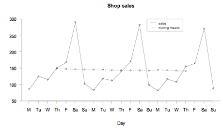
Daily sales, in thousands of dollars, for a hardware store were recorded for 21 days. There is reasonably systematic variation over each 7-day period, so moving means of order 7 have been calculated to attempt to eliminate this seasonal component. The moving mean for the first Thursday is calculated by (86 + 125 + 115 + 150 + 168 + 291 + 102)/7 = 148.14
Hardware store sales per day, with moving mean
| Mon
| 86
|
|
| Tue
| 125
|
|
| Wed
| 115
|
|
| Thu
| 150
| 148.14
|
| Fri
| 168
| 147.71
|
| Sat
| 291
| 146.71
|
| Sun
| 102
| 146.29
|
| Mon
| 83
| 145.00
|
| Tue
| 118
| 145.43
|
| Wed
| 112
| 144.14
|
| Thu
| 141
| 143.71
|
| Fri
| 171
| 143.57
|
| Sat
| 282
| 143.43
|
| Sun
| 99
| 142.86
|
| Mon
| 82
| 144.86
|
| Tue
| 117
| 144.00
|
| Wed
| 108
| 142.43
|
| Thu
| 155
| 140.86
|
| Fri
| 165
|
|
| Sat
| 271
|
|
| Sun
| 88
|
|
The raw data and the moving means are displayed below.

If you cannot view or read this graph, select this link to
open a text version.
Example 2 (quarterly data)
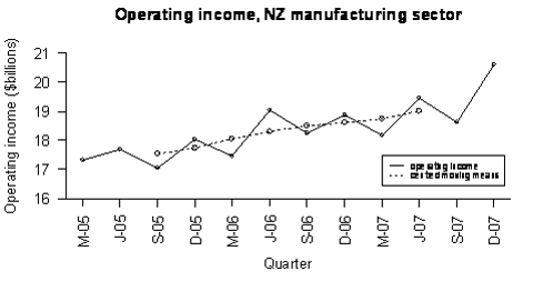
Statistics New Zealand’s Economic Survey of Manufacturing provided the following data on actual operating income for the manufacturing sector in New Zealand. There is reasonably systematic variation over each 4-quarter period, so moving means of order 4 have been calculated to attempt to eliminate this seasonal component. However, these moving means do not align with the quarters; the moving means are not centred. To align the moving means with the quarters, each pair of moving means is averaged to form centred moving means.
The first moving mean (between Mar-05 and Dec-05) is calculated by (17322 + 17696 + 17060 + 18046)/4 = 17531.
The centred moving mean for Sep-05 is calculated by (17531 + 17565.5)/2 = 17548.25.
Quarterly operating income, NZ manufacturing sector, with moving mean and centred moving mean
| Mar-05
| 17322
|
|
|
|
|
|
|
|
| Jun-05
| 17696
|
|
|
|
|
| 17531.00
|
|
| Sep-05
| 17060
|
| 17548.250
|
|
|
| 17565.50
|
|
| Dec-05
| 18046
|
| 17732.750
|
|
|
| 17900.00
|
|
| Mar-06
| 17460
|
| 18048.125
|
|
|
| 18196.25
|
|
| Jun-06
| 19034
|
| 18298.750
|
|
|
| 18401.25
|
|
| Sep-06
| 18245
|
| 18490.500
|
|
|
| 18579.75
|
|
| Dec-06
| 18866
|
| 18633.500
|
|
|
| 18687.25
|
|
| Mar-07
| 18174
|
| 18735.750
|
|
|
| 18784.25
|
|
| Jun-07
| 19464
|
| 19003.000
|
|
|
| 19221.75
|
|
| Sep-07
| 18633
|
|
|
| Dec-07
| 20616
|
|
|
The raw data and the centred moving means are displayed below. Note that M, J, S, and D indicate quarter years ending in March, June, September, and December respectively.

If you cannot view or read this graph, select this link to
open a text version.
See: moving average
Curriculum achievement objectives reference
Statistical investigation: (Level 8)
Multivariate data
A data set that has several variables.
Example
A data set consisting of the heights, ages, genders, and eye colours of a class of year 9 students.
Curriculum achievement objectives references
Statistical investigation: Levels 3, 4, 5, (6), (7), (8)
Mutually exclusive events
Events that cannot occur together.
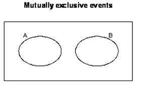
If events A and B are mutually exclusive, then the combined eventA and B contains no outcomes.

If you cannot view or read this graph, select this link to
open a text version.
Example 1
Suppose we have a group of men and women, and each is a possible outcome of a probability activity. If A is the event that a person is aged less than 30 years and B is the event that a person is aged over 50, the event A and B contains no outcomes because none of the people can be aged less than 30 years and over 50. Events A and B are therefore mutually exclusive.
Example 2
Consider rolling two dice. Suppose that event C consists of outcomes that have a total of 8 and that event D consists of outcomes with the first die showing a 1.
First explanation: If the first die shows a 1 (event D has occurred), then the greatest total for the two dice is 1 + 6 = 7, meaning that a total of 8 cannot occur. In other words, event C cannot occur together with event D.
Second explanation: C consists of the outcomes (2, 6), (3, 5), (4, 4), (5, 3), (6, 2), where (2, 6) means a 2 on the first die and a 6 on the second. D consists of the outcomes (1, 1), (1, 2), (1, 3), (1, 4), (1, 5), (1, 6). No outcomes are common to both event C and event D.
Events C and D are therefore mutually exclusive.
Alternative: disjoint events
Curriculum achievement objectives reference
Probability: Level (8)
Last updated October 16, 2013
TOP


