Glossary page P
Parameter
See: parameter(s) (of a theoretical distribution), population parameter
Parameter(s) (of a theoretical distribution)
A number (or numbers) occurring in the expression for a probability function or probability density function representing a theoretical distribution which, when changed, produce different members of the family of distributions. A given value for a parameter (or set of values for the parameters) determines a unique member of the family of distributions.
Example
The parameters of the binomial distribution are n and π.
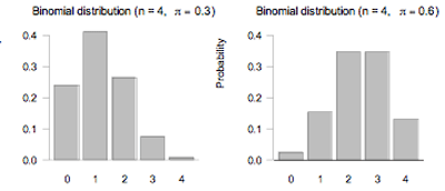
The graphs of the probability functions of two binomial distributions are shown below, one with n = 4 and π = 0.3 and the other with n = 4 and π = 0.6.
If you cannot view or read these graphs, select this link to
open a text version.
Curriculum achievement objectives references
Probability: Levels (7), (8)
Patterns
Regularities among distributions or regularities within a distribution. For sample distributions, a pattern should be a characteristic that would still be present if another sample were taken from the same population or if the current sample were enlarged by sampling further individuals from the same population.
Curriculum achievement objectives references
Statistical investigation: Levels 3, 4, 5, (6), (7), (8)
Picture graph
A graph for displaying the distribution of a category variable or a whole-number variable that uses pictures or symbols to represent the frequency of each category or value.
Picture graphs are useful for showing differences in frequency.
Example
A student collected data on the colour of cars that drove past her house and displayed the results on the picture graph below.
Picture graph: car colours
|
| red
|

|
|
| Grey/silver
|


|
| Colour
| Gold
|


|
|
| Green
|


|
|
| Blue
|


|
|
| White
|


|
If you cannot view or read this table, select this link to
open a text version.
Alternative: pictogram, pictograph
Curriculum achievement objectives references
Statistical investigation: Levels (2), (3), (4), (5)
Pie graph
There are two uses of pie graphs.
First, for displaying the relative frequency distribution of a category variable in which a circle is divided into sectors, representing categories, so that the area of each sector represents the relative frequency of values in the category. See Example 1 below.
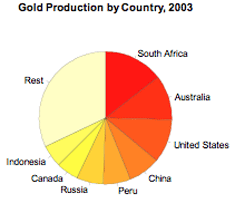
Second, for displaying bivariate data; one category variable and one numerical variable. A circle is divided into sectors, representing categories, so that the area of each sector represents the value of the numerical variable for the sector as a percentage of the total value for all sectors. See Example 2 below.
For categories that do not have a natural ordering, it is desirable to order the categories from the largest sector area to the smallest.
Example 1
Students enrolled in an introductory statistics course at the University of Auckland were asked to complete an online questionnaire. One of the questions asked them to enter their ethnicity. They chose from the following list: Chinese, Indian, Korean, Māori, New Zealand European, Other European, Pacific, Other. The 727 responses are displayed on the pie graph below.

If you cannot view or read this graph, select this link to
open a text version.
Example 2
World gold mine production for 2003 by country, based on official exports, is displayed on the bar graph below.
If you cannot view or read this graph, select this link to
open a text version.
Alternatives: circle graph, pie chart
Curriculum achievement objectives references
Statistical investigation: Levels (4), (5), (6), (7), (8)
Pilot survey
A trial run of the entire survey process using a small sample selected from the population. Its purpose is to identify any problems before the main survey begins.
Curriculum achievement objectives reference
Statistical investigation: (Level 7)
Placebo
A neutral treatment in an experiment that, to a person participating in the study, appears the same as the actual treatment.
Placebos are given to people in the control group so that reliable comparisons can be made between the treatment and control groups. People can experience positive outcomes from the psychological effect of believing they will improve because they have been given a treatment; the placebo effect. As part of determining whether a treatment is successful, researchers need to be able to see whether the effect due to a treatment is greater than the placebo effect.
Curriculum achievement objectives references
Statistical investigation: Levels (7), (8)
Statistical literacy: (Level 8)
Point estimate
A number calculated from a random sample that is used as an approximate value for a population parameter.
Example
A sample proportion, calculated from a random sample taken from a population, is a point estimate of the population proportion.
Alternative: estimate
See: interval estimate
Curriculum achievement objectives references
Statistical investigation: Levels (6), 7, (8)
Poisson distribution
A family of theoretical probability distributions, members of which may be useful as a model for some discrete random variables. Each distribution in this family gives the probability of obtaining a specified number of occurrences of a phenomenon in a specified interval in time or space, under the following conditions:
- On average, the phenomenon occurs at a constant rate, λ
- Occurrences of the phenomenon are independent of each other
- Two occurrences of the phenomenon cannot happen at exactly the same time or in exactly the same place.
A discrete random variable arising from a situation that closely matches the above conditions can be modelled by a Poisson distribution.
Each member of this family of distributions is uniquely identified by specifying the constant rate, λ. As such, λ, is the parameter of the Poisson distribution and the distribution is sometimes written as Poisson(λ).
Let random variableX represent the number of occurrences of a phenomenon that satisfies the conditions stated above. The probability of x occurrences is calculated by:
P(X = x) =
 for x = 0, 1, 2, ...
Example
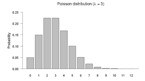
A graph of the probability function for the Poisson distribution with λ = 3 is shown below.
If you cannot view or read this graph, select this link to
open a text version.
Curriculum achievement objectives reference
Probability: Level 8
Poll
A systematic collection of data about opinions on issues taken by questioning a sample of people taken from a population in order to determine the opinion distribution of the population.
Alternative: opinion poll
See: survey
Curriculum achievement objectives references
Statistical investigation: Levels (5), (6), (7), (8)
Statistical literacy: Levels 7, 8
Population
A collection of all objects or individuals of interest that have properties that someone wishes to record.
Sometimes a population is a collection of potential objects or individuals and, as such, does not physically exist but can be imagined to exist.
Example 1 (A real population)
All people aged 18 and over who were living in New Zealand on 8 November 2008.
Example 2 (An imagined population)
All possible 15-watt fluorescent light bulbs that could be produced by a manufacturing plant.
Curriculum achievement objectives references
Statistical investigation: Levels 6, 7, (8)
Population distribution
The variation in the values of a variable if data has (or had) been obtained for every individual in the population.
For a numerical variable, if the values are whole numbers, a population distribution may be displayed:
- in a table, as a set of values and their corresponding frequencies,
- in a table, as a set of values and their corresponding proportions or probabilities, or
- on an appropriate graph such as a bar graph.
For a numerical variable, if the values are measurements, a population distribution may be displayed:
- in a table, as a set of class intervals and their corresponding frequencies,
- in a table, as a set of class intervals and their corresponding proportions or probabilities, or
- on an appropriate graph such as a histogram, stem-and-leaf plot, box and whisker plot or dot plot.
For a category variable, a population distribution may be displayed:
- in a table, as a set of categories and their corresponding frequencies,
- in a table, as a set of categories and their corresponding proportions or probabilities, or
- on an appropriate graph such as a bar graph.
See: distribution
Curriculum achievement objectives references
Statistical investigation: Levels (5), (6), (7), (8)
Probability: Levels (5), (6), (7), (8)
Population mean
A measure of centre for a population distribution of a numerical variable. The population mean is the mean of all values of a numerical variable based on the collection of all objects or individuals of interest. It is the centre of mass of the values in a population distribution.
If the collection is finite then the population mean is obtained by adding all values in a set of values and then dividing this total by the number of values.
In many real situations, the entire collection of values from a population is not available, for a variety of reasons. For example, the collection may be infinite or some objects or individuals may not be accessible. In such cases, the value of the population mean is not known. The population mean may be estimated by taking a random sample of values from the population, calculating the sample mean and using this value as an estimate of the population mean.
The population mean is a number representing the centre of the population distribution and is therefore an example of a population parameter.
The Greek letter µ (mu) is the most common symbol for the population mean.
See: expected value (of a discrete random variable), mean, measure of centre
Curriculum achievement objectives references
Statistical investigation: Levels (6), (7), (8)
Population parameter
A number representing a property of a population.
Common examples are the population mean, µ, the population proportion, π, and the population standard deviation, σ.
Population parameters, although fixed, are usually not known and are estimated by a statistic calculated from a random sample taken from the population. For example, a sample mean is an estimate of the population mean.
Curriculum achievement objectives references
Statistical investigation: Levels 7, (8)
Population proportion
A part of a population with a particular attribute, expressed as a fraction, decimal, or percentage of the whole population.
For a finite population, the population proportion is the number of members in the population with a particular attribute divided by the number of members in the population.
In many real situations, the whole population is not available to be checked for the presence of an attribute. In such cases, the value of the population proportion is not known. The population proportion may be estimated by taking a random sample from the population, calculating the sample proportion and using this value as an estimate of the population proportion.
The population proportion is a number representing a part of a population and is therefore an example of a population parameter.
The Greek letter π (pi) is a common symbol for the population proportion.
See: proportion
Curriculum achievement objectives references
Statistical investigation: Levels (7), (8)
Population standard deviation
A measure of spread for a population distribution of a numerical variable that determines the degree to which the values differ from the population mean. If many values are close to the population mean, then the population standard deviation is small, and if many values are far from the population mean, then the population standard deviation is large.
The square of the population standard deviation is equal to the population variance.
In many real situations, the collection of all values from a population is not available for a variety of reasons. For example, the collection may be infinite or some objects or individuals may not be accessible. In such cases, the value of the population standard deviation is not known. The population standard deviation may be estimated by taking a random sample of values from the population, calculating the sample standard deviation and using this value as an estimate of the population standard deviation.
The population standard deviation is a number representing the spread of the population distribution and is therefore an example of a population parameter.
The Greek letter σ (sigma) is the most common symbol for the population standard deviation.
See: measure of spread, population variance, standard deviation, standard deviation (of a discrete random variable)
Curriculum achievement objectives references
Statistical investigation: Levels (7), (8)
Population variance
A measure of spread for a population distribution of a numerical variable that determines the degree to which the values differ from the population mean. If many values are close to the population mean, then the population variance is small, and if many values are far from the population mean, then the population variance is large.
The positive square root of the population variance is equal to the population standard deviation.
In many real situations, the collection of all values from a population is not available for a variety of reasons. For example, the collection may be infinite or some objects or individuals may not be accessible. In such cases, the value of the population variance is not known. The population variance may be estimated by taking a random sample of values from the population, calculating the sample variance and using this value as an estimate of the population variance.
The population variance is a number representing the spread of a population and is therefore an example of a population parameter.
The square of the population standard deviation is equal to the population variance, so σ2 (sigma squared) is the most common symbol for the population variance.
See: measure of spread, variance, variance (of a discrete random variable)
Curriculum achievement objectives references
Statistical investigation: Levels (7), (8)
Precision (of an estimate)
A measure of how close an estimate is expected to be to the true value of a population parameter. This measure is based on the degree of similarity among estimates of a population parameter if the same sampling method were repeated over and over again.
Curriculum achievement objectives references
Statistical investigation: Levels (7), 8
Statistical literacy: (Level 8)
Prediction
An assessment of the value of a variable at some future point of time (for time-series data) or, in linear regression on numerical bivariate data, an assessment of the value of one numerical variable based on the value of the other numerical variable.
See: estimate, forecast
Curriculum achievement objectives references
Statistical investigation: Levels 7, 8
Probabilistic model
A model that takes uncertainty in outcomes into account. This is often done by associating a probability with each possible outcome. A probabilistic model includes elements of randomness. A model, being an idealised description of a situation, is developed by making some assumptions about that situation.
Example
A probabilistic model for flipping two fair coins and observing the number of heads facing upwards:
The sample space is: 0 heads, 1 head, 2 heads
Assuming that each flip is independent of all other flips and that the probability of each coin turning up a head is the same for each flip, the probability of each outcome is:
P(no heads) = 1/4
P(1 head) = 1/2
P(2 heads) = 1/4
Note that if two fair coins are flipped the outcome cannot be predicted with certainty.
See: deterministic model
Curriculum achievement objectives reference
Probability: (Level 8)
Probability
A number that describes the likely occurrence of an event, measured on a scale from 0 (impossible event) to 1 (certain event).
Curriculum achievement objectives references
Statistical literacy: Level 6
Probability: Levels 4, 5, 6, 7, 8
Probability activity
An activity that has a number of possible outcomes, none of which is certain to occur when a trial of the activity is performed.
Curriculum achievement objectives references
Statistical literacy: Levels 1, 2, 3, 4, 5
Probability: (All levels)
Probability density function (for a continuous random variable)
A mathematical function that provides a model for the probability that a value of a continuous random variable lies within a particular interval. A probability density function is a theoretical probability distribution for a continuous random variable.
A probability density function is often displayed as a graph, in which case the probability is the area between the graph of the function and the x-axis, bounded by the particular interval.
A probability density function has two further important properties:
- Values of a probability density function are never negative for any value of the random variable.
- The area under the graph of a probability density function is 1.
The use of ‘density’ in this term relates to the height of the graph. The height of the probability density function represents how closely the values of the random variable are packed at places on the x-axis. At places on the x-axis where the values are closely packed (dense) the height is greater than at places where the values are not closely packed (sparse).
More formally, probability density represents the probability per unit interval on the x-axis.
Example
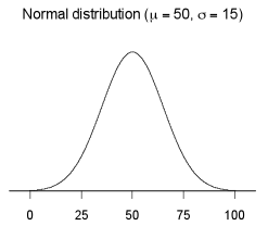
Let X be a random variable with a normal distribution with a mean of 50 and a standard deviation of 15. The graph below shows the probability density function of X.
If you cannot view or read this graph, select this link to
open a text version.
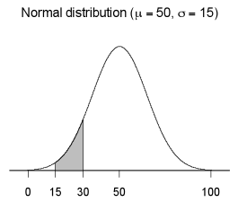
On the diagram below the shaded area equals the probability that X is between 15 and 30, that is, P(15 < X < 30).
If you cannot view or read this graph, select this link to
open a text version.
Alternative: probability model
See: normal distribution, triangular distribution, uniform distribution (for a continuous variable),
Curriculum achievement objectives references
Probability: Levels (7), (8)
Probability distribution
The variation in the values of a variable in which the method of displaying this variation uses probabilities.
For a whole-number variable or discrete variable, a probability distribution may be:
- displayed in a table, as a set of values and their corresponding probabilities,
- displayed on an appropriate graph such as a bar graph, or
- represented as a mathematical function (at Level 6 or above).
For measurement data, a probability distribution may be:
- displayed in a table, as a set of intervals of values (class intervals) and their corresponding probabilities,
- displayed on an appropriate graph such as a histogram, or
- represented as a probability density function when it is a theoretical probability distribution (at Levels 7 or 8, as a mathematical function or graph).
For category data, a probability distribution may be:
- displayed in a table, as a set of categories and their corresponding probabilities, or
- on an appropriate graph such as a bar graph.
The probabilities may come from a variety of sources such as a sample, experiment, population or model.
Probability distributions arising from a model are examples of theoretical probability distributions.
See: distribution
Curriculum achievement objectives references
Statistical investigation: (Level 8)
Probability: Levels (5), (6), (7), (8)
Probability function (for a discrete random variable)
A mathematical function that provides a model for the probability of each value of a discrete random variable occurring. A probability function is a theoretical probability distribution for a discrete random variable.
For a discrete random variable that has a finite number of possible values, the function is sometimes displayed as a table, listing the values of the random variable and their corresponding probabilities.
A probability function has two important properties:
- For each value of the random variable, values of a probability function are never negative, nor greater than 1.
- The sum of the values of a probability function, taken over all of the values of the random variable, is 1.
Example 1
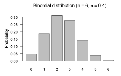
Let X be a random variable with a binomial distribution with n = 6 and π = 0.4. The probability function for random variable X is:
Probability of x successes in 6 trials, P(X = x) =
 for x = 0, 1, 2, 3, 4, 5, 6
If you cannot view or read this formula, select this link to
open a text version.
where
 is the number of combinations of n objects taken x at a time.
If you cannot view or read this formula, select this link to
open a text version.
A graph of this probability function is shown below.

If you cannot view or read this graph, select this link to
open a text version.
Example 2
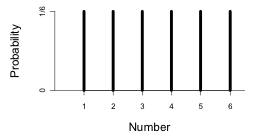
Imagine a probability activity in which a fair, six-faced die will be rolled and the number facing upwards recorded. Let random variable X represent the result of any roll.
The probability function for random variable X can be written as:
Probabilities for a fair six-sided die.
| X
| 1
| 2
| 3
| 4
| 5
| 6
|
| P(X=x)
| 1/6
| 1/6
| 1/6
| 1/6
| 1/6
| 1/6
|
and graphed as:

If you cannot view or read this graph, select this link to
open a text version.
This model assumes that each roll is independent of all other rolls and that the probability of each number facing upwards is the same for each roll.
Alternative: probability model
See: binomial distribution, model, uniform distribution (for a whole-number or discrete variable)
Curriculum achievement objectives references
Probability: Levels (7), (8)
Proportion
A part of a distribution with a particular attribute, expressed as a fraction, decimal, or percentage of the whole distribution.
See: sample proportion
Curriculum achievement objectives references
Statistical investigation: Levels 5, (6), (7), 8
Last updated October 16, 2013
TOP


 for x = 0, 1, 2, 3, 4, 5, 6