Glossary page S
Sample
A group of objects, individuals, or values selected from a population. The intention is for this sample to provide estimates of population parameters.
See: cluster sampling, random sample, simple random sample, stratified sampling, systematic sampling
Curriculum achievement objectives references
Statistical investigation: Levels 5, (6), (7), (8)
Probability: Levels 6, (7)
Sample distribution
The variation in the values of a variable in data obtained from a sample.
For whole-number data, a sample distribution may be displayed:
- in a table, as a set of values and their corresponding frequencies,
- in a table, as a set of values and their corresponding proportions, or
- on an appropriate graph such as a bar graph.
For measurement data, a sample distribution may be displayed:
- in a table, as a set of intervals of values (class intervals) and their corresponding frequencies,
- in a table, as a set of intervals of values (class intervals) and their corresponding proportions, or
- on an appropriate graph such as a histogram, stem-and-leaf plot, box and whisker plot or dot plot.
For category data, a sample distribution may be displayed:
- in a table, as a set of categories and their corresponding frequencies,
- in a table, as a set of categories and their corresponding proportions, or
- on an appropriate graph such as a bar graph.
A sample distribution is sometimes called an experimental distribution.
Alternative: empirical distribution
See: distribution, experimental distribution
Curriculum achievement objectives references
Statistical investigation: Levels 5, (6), (7), (8)
Sample mean
A measure of centre for the distribution of a sample of numerical values. The sample mean is the centre of mass of the values in their distribution.
If the n values in a sample are x1, x2, ... , xn, then the sample mean is calculated by adding the values in the sample and then dividing this total by the number of values. In symbols, the sample mean,
 , is calculated by
 =
=
 .
.
For large samples, it is recommended that a calculator or software is used to calculate the mean.
The sample mean is a (sample) statistic and is therefore an estimate of the population mean.
See: mean
Curriculum achievement objectives references
Statistical investigation: Levels (6), (7), (8)
Sample proportion
A part of a sample with a particular attribute, expressed as a fraction, decimal, or percentage of the whole sample.
A common symbol for the sample proportion is p.
Example
Suppose the attribute of interest was left-handedness and that a random sample of 10 people contained 3 left-handed people.
The sample proportion is 3/10 or 0.3 or 30%.
See: proportion
Curriculum achievement objectives references
Statistical investigation: Levels (6), (7), 8
Sample size
The number of objects, individuals, or values in a sample.
Typically, a larger sample size leads to an increase in the precision of a statistic as an estimate of a population parameter.
The most common symbol for sample size is n.
Curriculum achievement objectives references
Statistical investigation: Levels (5), (6), 7, (8)
Probability: Levels 6, (7)
Sample space
The set of all of the possible outcomes for a probability activity or a situation involving an element of chance.
For discrete situations, the sample space can be listed.
Note that a sample space can often be described in several different ways.
Example 1
In a situation where a person will be selected and their eye colour recorded, a sample space is blue, grey, green, hazel, brown. Each person’s eye colour must belong to exactly one of these categories.
Example 2
In a situation where the gender of the child is recorded in birth order, a sample space is (BBB, BBG, BGB, BGG, GBB, GBG, GGB, GGG).
A different sample space could be 3 boys, exactly 2 boys, exactly 1 boy, no boys.
A different sample space again could be more boys than girls, more girls than boys.
Curriculum achievement objectives references
Probability: Levels (4), (5), (6), (7), 8
Sample standard deviation
A measure of spread for a distribution of a sample of numerical values that determines the degree to which the values differ from the sample mean.
It is calculated by taking the square root of the average of the squares of the deviations of the values from their sample mean.
It is recommended that a calculator or software is used to calculate the sample standard deviation.
The square of the sample standard deviation is equal to the sample variance.
A common symbol for the sample standard deviation is s.
The sample standard deviation is a (sample) statistic and is therefore an estimate of the population standard deviation.
See: measure of spread, sample variance, standard deviation
Curriculum achievement objectives references
Statistical investigation: Levels (6), (7), (8)
Sample statistic
A number that is calculated from a sample of numerical values.
A sample statistic gives an estimate of the corresponding value from the population from which the sample was taken. For example, a sample mean is an estimate of the population mean.
See: statistic
Curriculum achievement objectives references
Statistical investigation: Levels (6), 7, (8)
Sample statistics
Numbers calculated from a sample of numerical values that are used to summarise the sample. The statistics will usually include at least one measure of centre and at least one measure of spread.
Alternative: numerical summary
See: descriptive statistics, summary statistics
Curriculum achievement objectives references
Statistical investigation: Levels (6), (7), (8)
Sample variance
A measure of spread for a distribution of a sample of numerical values that determines the degree to which the values differ from the sample mean.
It is calculated by the average of the squares of the deviations of the values from their sample mean.
The positive square root of the sample variance is equal to the sample standard deviation.
It is recommended that a calculator or software is used to calculate the sample variance. On a calculator, the square of the standard deviation will give the variance.
A common symbol for the sample variance is s2.
The sample variance is a (sample) statistic and is therefore an estimate of the population variance.
See: measure of spread, sample standard deviation, variance
Curriculum achievement objectives references
Statistical investigation: Levels (7), (8)
Sampling distribution
A distribution for the variation in the values of a statistic, such as a sample mean, produced by repeated sampling. When the statistic is the sample mean, the sampling distribution is called the sampling distribution of the sample mean.
At level 8 a bootstrap distribution for an estimate or statistic is an approximation to the sampling distribution for the estimate or statistic.
Example 1
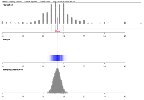
The ‘sampling variation’ module from the
iNZightVIT software, produced the following output. Note that to use this module you must have data on every unit in the population.

If you cannot view or read this diagram/graph, select this link to
open a text version.
The population used is 500 students from the CensusAtSchool database. This is multivariate data. The variable ‘rightfoot’ (the length of a student’s right foot, in centimetres), the quantity ‘mean’, the sample size ‘25’ and the number of repetitions ‘1000’ were selected.
The ‘Population’ plot shows the population distribution of the right foot lengths of the 500 students in the population.
In the ‘Sample’ plot, each vertical line represents a sample mean calculated from a random sample of 25 students from the population.
In the ‘Sampling Distribution’ plot, each dot represents a sample mean calculated from a random sample of 25 students from the population. 1000 dots are displayed; one for each sample mean. The plot shows a sampling distribution of the sample mean.
Example 2
Consider the mean of a random sample of 20 values taken from a population. Suppose that several more random samples of 20 values were taken from the same population and the sample mean for each sample was calculated. The values of these sample means would differ from sample to sample (illustrating sampling variation). Imagine repeating this process over and over again, without end. The variation in the values of these sample means is the sampling distribution of the sample mean. This is an example of a theoretical sampling distribution.
See: central limit theorem, distribution
Curriculum achievement objectives reference
Statistical investigation: Level 8
Sampling error
The error that arises in a data collection process as a result of taking a sample from a population rather than using the whole population.
Sampling error is one of two reasons for the difference between an estimate of a population parameter and the true, but unknown, value of the population parameter. The other reason is non-sampling error. Even if a sampling process has no non-sampling errors then estimates from different random samples (of the same size) will vary from sample to sample, and each estimate is likely to be different from the true value of the population parameter.
The sampling error for a given sample is unknown but when the sampling is random, for some estimates (for example, sample mean, sample proportion) theoretical methods may be used to measure the extent of the variation caused by sampling error.
See: margin of error, non-sampling error, standard error
Curriculum achievement objectives references
Statistical investigation: Levels (7), (8)
Statistical literacy: Levels 7, (8)
Sampling variation
The variation in a sample statistic from sample to sample.
Suppose a sample is taken and a sample statistic, such as a sample mean, is calculated. If a second sample of the same size is taken from the same population, it is almost certain that the sample mean calculated from this sample will be different from that calculated from the first sample. If further sample means are calculated, by repeatedly taking samples of the same size from the same population, then the differences in these sample means illustrate sampling variation.
Alternative: chance variation
Curriculum achievement objectives references
Statistical investigation: Levels (5), (6), (7), (8)
Probability: Levels (3), (4), (5), (6)
Scatter
For bivariate numerical data, the variation (in the vertical direction) of the values of the variable plotted on the y-axis of a scatter plot.
In linear regression, scatter is the variation (in the vertical direction) of the values of the response variable from the regression line.
Curriculum achievement objectives reference
Statistical investigation: (Level 8)
Scatter plot
A graph for displaying a pair of numerical variables. The graph has two axes, one for each variable, and points are plotted to show the values of these two variables for each of the individuals.
A scatter plot is essential for exploring the relationship that may exist between the two variables and for revealing the features of this relationship.
In linear regression, at level 8, one of the two variables is regarded as the explanatory variable and the other variable as the response variable. In this case, the explanatory variable is plotted on the horizontal axis (x-axis) and the response variable is plotted on the vertical axis (y-axis).
When fitting models to data, as in linear regression, a scatter plot is essential for assessing how useful the fitted model may be.
Example
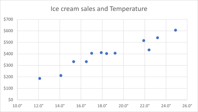
In this hypothetical example, ice cream sales (in dollars) and temperature in (degrees) are displayed on the scatter plot below.
If you cannot view or read this graph, select this link to
open a text version.
Alternatives: scatter diagram, scattergram, scatter graph
Curriculum achievement objectives references
Statistical investigation: Levels (4), (5), (6), (7), (8)
Seasonal component (for time-series data)
Variations in time-series data that repeat more or less regularly, which are due to the effect of the seasons of the year, or to the effect of other periodic influences such as systematic patterns within each week or within each day.
Alternative: seasonality
See: time-series data
Curriculum achievement objectives reference
Statistical investigation: Level (8)
Seasonally adjusted data
Time-series data which have had the seasonal component removed. In seasonally adjusted data, the effect of regular seasonal phenomena has been removed.
In terms of an additive model for time-series data, Y = T + S + C + I, where
T represents the trend component,
S represents the seasonal component,
C represents the cyclical component, and
I represents the irregular component;
the smoothed series = T + C and
the seasonally adjusted series = T + C + I.
Example
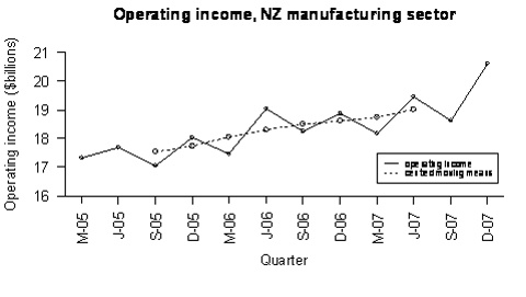
Statistics New Zealand’s Economic Survey of Manufacturing provided the following data on actual operating income for the manufacturing sector in New Zealand. Centred moving means have been calculated. For the quarters with centred moving means, the individual seasonal effect is calculated by:
Operating income (raw data) – (centred) moving mean
The overall seasonal effect for each quarter is estimated by averaging the individual seasonal effects. The two individual seasonal effects for March quarters are –588.125 and –561.75. The mean of these 2 values is –574.938. The other estimated overall seasonal effects are shown in the second table below.
Seasonally adjusted data is calculated by:
Operating income (raw data) – estimated overall seasonal effect
The calculation for the Mar-05 quarter is 17322 – (–574.938) = 17896.938.
Seasonally adjusted operating income, NZ manufacturing sector.
| Mar-05
| 17322
|
|
| 17896.938
|
| Jun-05
| 17696
|
|
| 17097.875
|
| Sep-05
| 17060
| 17548.250
| -488.250
| 17426.875
|
| Dec-05
| 18046
| 17732.750
| 313.250
| 17773.125
|
| Mar-06
| 17460
| 18048.125
| -588.125
| 18034.938
|
| Jun-06
| 19034
| 18298.750
| 735.250
| 18435.875
|
| Sep-06
| 18245
| 18490.500
| -245.500
| 18611.875
|
| Dec-06
| 18866
| 18633.500
| 232.500
| 18593.125
|
| Mar-07
| 18174
| 18735.750
| -561.750
| 18748.938
|
| Jun-07
| 19464
| 19003.000
| 461.000
| 18865.875
|
| Sep-07
| 18633
|
|
| 18999.875
|
| Dec-07
| 20616
|
|
| 20343.125
|
Seasonal effects on operating income by quarter, NZ manufacturing sector.
|
| Mar
| Jun
| Sep
| Dec
|
| Individual
| -588.125
| 735.250
| -488.250
| 313.250
|
| -561.750
| 461.000
| -245.500
| 232.500
|
| Overall
| -574.938
| 598.125
| -366.875
| 272.875
|
The raw data and the seasonally adjusted data are displayed below. Note that M, J, S, and D indicate quarter years ending in March, June, September, and December respectively.

If you cannot view or read this graph, select this link to
open a text version.
Curriculum achievement objectives reference
Statistical investigation: Level (8)
Simple random sample
A sample in which, at any stage of the sampling process, each object or individual (which has not been chosen) in the population has the same probability of being chosen in the sample.
In a simple random sample, an object or individual in the population can be chosen once at most. This is often called sampling without replacement.
See: random sample
Curriculum achievement objectives references
Statistical investigation: Levels (6), (7), (8)
Simulation
A technique for imitating the behaviour of a situation that involves elements of chance or a probability activity. The technique uses tools such as coins, dice, random numbers from a calculator, random numbers from random number tables, and random numbers generated by computers.
Example 1
A coin can be used to simulate the outcomes of three-child families, assuming that a boy and a girl are equally likely to occur. If a head results from the coin toss, then a boy is the simulated birth outcome, and if a tail results, then a girl is the simulated birth outcome. A group of three coin tosses simulates an outcome of a three-child family. The simulation is continued until the required number of trials has been performed.
Suppose the results of 90 coin tosses and therefore 30 simulated trials of three-child families were:
HHT TTT HHT HTT HHT TTT THT TTH THT THT THT TTT HTH HTH HHH THT THT THH TTT HHH HHT TTH THT THH HTT THH THT HTH THH HHH
Trials:
BBG GGG BBG BGG BBG GGG GBG GGB GBG GBG GBG GGG BGB BGB BBB GBG GBG GBB GGG BBB BBG GGB GBG GBB BGG GBB GBG BGB GBB BBB
The experimental distribution for the variable that lists numbers of boys and girls in the family is shown in the frequency table or one-way table below.
Frequency of gender combinations for three-child families.
| Combination
| 3 boys
| 2 boys and 1 girl
| 1 boy an 2 girls
| 3 girls
|
| Frequency
| 3
| 11
| 12
| 4
|
Example 2
In a game of tennis, one player from School A is to play one player from School B. School A has 3 players to choose from (C, D, and E) and School B has 2 players to choose from (F and G). For School A, the probabilities of C, D, or E being selected are 0.6, 0.3, and 0.1 respectively. For school B, the probabilities of F or G being selected are 0.7 and 0.3 respectively.
Simulate 25 performances (or trials) of this activity.
Suppose the random numbers to be used, starting at the beginning of this list, were
71578 81355 39007 60764 19852 87652 50354 22183 14935 09519
Consider the digits in pairs.
The first digit will decide the player for School A. If it is 0, 1, 2, 3, 4, or 5, then player C is chosen; if it is 6, 7, or 8, then player D is chosen; if it is 9, then player E is chosen.
The second digit will decide the player for School B. If it is 0, 1, 2, 3, 4, 5, or 6, then player F is chosen; if it is 7, 8, or 9, then player G is chosen.
Simulation results for inter-school tennis player selection.
| 1
| 71
| D plays F
| 14
| 76
| D plays F
|
| 2
| 57
| C plays G
| 15
| 52
| C plays F
|
| 3
| 88
| D plays G
| 16
| 50
| C plays F
|
| 4
| 13
| C plays F
| 17
| 35
| C plays F
|
| 5
| 55
| C plays F
| 18
| 42
| C plays F
|
| 6
| 39
| C plays G
| 19
| 21
| C plays F
|
| 7
| 00
| C plays F
| 20
| 83
| D plays F
|
| 8
| 76
| D plays F
| 21
| 14
| C plays F
|
| 9
| 07
| C plays G
| 22
| 93
| E plays F
|
| 10
| 64
| D plays F
| 23
| 50
| C plays F
|
| 11
| 19
| C plays G
| 24
| 95
| E plays F
|
| 12
| 85
| D plays F
| 25
| 19
| C plays G
|
| 13
| 28
| C plays G
|
|
|
|
The experimental distribution for the variable that lists pairs of players is shown in the frequency table or one-way table below.
Frequency of inter-school tennis player selections.
| Combination
| C plays F
| C plays G
| D plays F
| D plays G
| E plays F
| E plays G
|
| Frequency
| 10
| 6
| 6
| 1
| 2
| 0
|
Curriculum achievement objectives references
Probability: Levels 7, (8)
Skewness
A lack of symmetry in a distribution of a numerical distribution in which the values on one side of the distribution tend to be further from the centre of the distribution than values on the other side.
If the smaller values of a distribution tend to be further from the centre of the distribution than the larger values, the distribution is said to have negative skew or to be skewed to the left (or left-skewed).
If the larger values of a distribution tend to be further from the centre of the distribution than the smaller values, the distribution is said to have positive skew or to be skewed to the right (or right-skewed).
Example 1
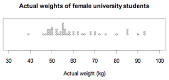
The actual weights of a random sample of 50 female university students enrolled in an introductory statistics course at the University of Auckland are displayed on the dot plot below. The sample distribution is skewed to the right or positively skewed.

If you cannot view or read this graph, select this link to
open a text version.
Example 2
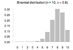
The bar graph displays the probability function of the binomial distribution with n = 10 and π = 0.8. The theoretical distribution is skewed to the left or negatively skewed.

If you cannot view or read this graph, select this link to
open a text version.
Curriculum achievement objectives references
Statistical investigation: Levels (4), (5), (6), (7), (8)
Smoothing data
A process of removing fluctuations from time-series data so that the resulting series shows much less variation, and is therefore smoother.
At level 8, moving averages (usually moving means) are used as a method of smoothing time-series data.
See: moving averages, moving mean, time-series data
Curriculum achievement objectives reference
Statistical investigation: (Level 8)
Sources of variation
The reasons for differences seen in the values of a variable. Some of these reasons are summarised in the following paragraphs.
Variation is present everywhere and is in everything. When the same variable is measured for different individuals, there will be differences in the measurements, simply due to the fact that individuals are different. This can be thought of as individual-to-individual variation and is often described as natural or real variation.
Repeated measurements on the same individual may vary because of changes in the variable being measured. For example, an individual’s blood pressure is not exactly the same throughout the day. This can be thought of as occasion-to-occasion variation.
Repeated measurements on the same individual may vary because of some unreliability in the measurement device, such as a slightly different placement of a ruler when measuring. This is often described as measurement variation.
The difference in measurements of the same quantity for different individuals, apart from natural variation, could be due to the effect of one or more other factors. For example, the difference in growth of two tomato plants from the same packet of seeds planted in two different places could be due to differences in the growing conditions at those places, such as soil fertility or exposure to sun or wind. Even if the two seeds were planted in the same garden, there could be differences in the growth of the plants due to differences in soil conditions within the garden. This is often described as induced variation.
Variation occurs in all sampling situations. Suppose a sample is taken and a sample statistic, such as a sample mean, is calculated. If a second sample of the same size is taken from the same population, it is almost certain that the sample mean calculated from this sample will be different from that calculated from the first sample. If further sample means are calculated, by repeatedly taking samples of the same size from the same population, then the differences in these sample means illustrate sampling variation.
Curriculum achievement objectives references
Statistical investigation: Levels 5, 6, (7), (8)
Spread
The degree to which values in a distribution of a numerical variable differ from one another.
Alternative: dispersion
See: variability, variation
Curriculum achievement objectives references
Statistical investigation: Levels 5, (6), (7), (8)
Standard deviation
A measure of spread for a distribution of a numerical variable that determines the degree to which the values differ from the mean. If many values are close to the mean, then the standard deviation is small, and if many values are far from the mean, then the standard deviation is large.
It is calculated by taking the square root of the average of the squares of the deviations of the values from their mean.
It is recommended that a calculator or software is used to calculate the standard deviation.
The standard deviation can be influenced by unusually large or unusually small values. It is recommended that a graph of the distribution is used to check the appropriateness of the standard deviation as a measure of spread and to emphasise its meaning as a feature of the distribution.
The square of the standard deviation is equal to the variance.
Note that calculators have two keys for the two different ways the standard deviation can be calculated. One way divides the sum of the squared deviations by the number of values before taking the square root. The other way divides the sum of the squared deviations by one less than the number of values before taking the square root. At school level, it does not really matter which key is used because for all but quite small data sets the two values for the standard deviation will be similar. Software tends to use the calculation that divides by one less than the number of values; but some offer both ways. The first way (dividing by the number of values) is better when there are values for all members of a population, and the second way is better when the values are from a sample.
Example
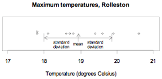
The maximum temperatures, in degrees Celsius (°C), in Rolleston for the first 10 days in November 2008 were 18.6, 19.9, 20.6, 19.4, 17.8, 18.1, 17.8, 18.7, 19.6, 18.8.
The standard deviation using division by 9 (one less than the number of values) is 0.93°C.
The standard deviation using division by 10 (the number of values) is 0.88°C.
The data, the mean, and the standard deviation are displayed on the dot plot below.

If you cannot view or read this graph, select this link to
open a text version.
See: measure of spread, population standard deviation, sample standard deviation, variance
Curriculum achievement objectives references
Statistical investigation: Levels (5), (6), (7), (8)
Standard deviation (of a discrete random variable)
A measure of spread for a distribution of a random variable that determines the degree to which the values differ from the expected value.
The standard deviation of random variable X is often written as σ or σX.
For a discrete random variable the standard deviation is calculated by summing the product of the square of the difference between the value of the random variable and the expected value, and the associated probability of the value of the random variable, taken over all of the values of the random variable, and finally taking the square root.
In symbols, σ =

An equivalent formula is, σ =
 .
.
The square of the standard deviation is equal to the variance, Var(X) = σ 2.
Example
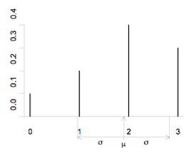
Random variable X has the following probability function:
probabilities for a random variable X.
| x
| 0
| 1
| 2
| 3
|
| P(X = x)
| 0.1
| 0.2
| 0.4
| 0.3
|
Using σ =

µ = 0 x 0.1 + 1 x 0.2 + 2 x 0.4 + 3 x 0.3
= 1.9
σ =

=

= 0.94
Using σ =

E(X) = 0 x 0.1 + 1 x 0.2 + 2 x 0.4 + 3 x 0.3
= 1.9
E(X2) = 02 × 0.1 + 12 × 0.2 + 22 × 0.4 + 32 × 0.3
= 4.5
σ =

= 0.94
A bar graph of the probability function, with the mean and standard deviation labelled, is shown below.

If you cannot view or read this graph, select this link to
open a text version.
See: population standard deviation, standard deviation
Curriculum achievement objectives reference
Probability: Level 8
Standard error
A measure of spread for the values of an estimate or statistic, based on considering the sampling being repeated over and over. As such, a standard error is a measure of the precision of an estimate or statistic.
Estimates vary from sample to sample. When considering the sampling being repeated over and over, infinitely, the sampling distribution of an estimate is a theoretical probability distribution for the variation in the estimate or statistic. Standard error is used with two similar, but different, meanings.
- The first meaning is the standard deviation of the (theoretical) sampling distribution of an estimate or statistic.
- The second meaning is an estimated standard deviation of the (theoretical) sampling distribution of an estimate.
The standard deviation of the sampling distribution of an estimate is usually unknown and so the second meaning is more useful.
For some statistics (for example, sample mean, sample proportion) theoretical methods may be used to find the standard error of an estimate but these methods are beyond Level 8 of the New Zealand Curriculum.
At Level 8 a bootstrap distribution for an estimate or statistic is an approximation to the sampling distribution for the estimate. The standard deviation of a bootstrap distribution gives an approximate value of the standard error.
Curriculum achievement objectives reference
Statistical investigation: (Level 8)
Standard normal distribution
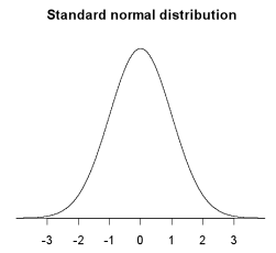
The normal distribution with a mean of 0 and a standard deviation of 1.
A graph of the probability density function for the standard normal distribution is shown below.

If you cannot view or read this graph, select this link to
open a text version.
Curriculum achievement objectives references
Probability: Levels (7), (8)
Statistic
A number that is calculated from numerical data.
Statistics listed in this glossary are mean, median, mode, standard deviation, variance, interquartile range, range, lower quartile, upper quartile.
Alternative: summary statistic
See: sample statistic
Curriculum achievement objectives references
Statistical investigation: Levels (6), (7), (8)
Statistical literacy: Levels 6, (7), (8)
Statistics
The process of finding out more about the real world by collecting and then making sense of data. (Reference: Chance Encounters, Wild, C.J. and Seber G.A.F., Wiley (2000), p 28)
Curriculum achievement objectives references
Statistical investigation: All levels
Statistical literacy: All levels
Probability: All levels
Statistical enquiry cycle
A cycle that is used to carry out a statistical investigation. The cycle consists of five stages: Problem, Plan, Data, Analysis, Conclusion. The cycle is sometimes abbreviated to the PPDAC cycle.
The problem section is about formulating a statistical question, what data to collect, who to collect it from, and why it is important.
The plan section is about how the data will be gathered.
The data section is about how the data is managed and organised.
The analysis section is about exploring and analysing the data, using a variety of data displays and numerical summaries, and reasoning with the data.
The conclusion section is about answering the question in the problem section and giving reasons based on the analysis section.
Reference:
How kids learn – the statistical enquiry cycle
Curriculum achievement objectives references
Statistical investigation: All levels
Statistical inference
The process of drawing conclusions about population parameters based on a sample taken from the population.
Example 1
Using a sample mean calculated from a random sample taken from a population to estimate the population mean is an example of statistical inference.
Example 2
Using data from a random sample taken from a population to obtain a 95% confidence interval for the population proportion is an example of statistical inference.
Alternative: inference
Curriculum achievement objectives references
Statistical investigation: Levels 6, 7, 8
Statistical investigation
An information gathering and learning process that is undertaken to seek meaning from and to learn more about any aspect of the real world, as well as to help make informed decisions and take informed actions. Statistical investigations should use the statistical enquiry cycle (Problem, Plan, Data, Analysis, Conclusion).
Reference:
Statistical Investigation (PDF)
See: statistical enquiry cycle
Curriculum achievement objectives references
Statistical investigation: All levels
Statistical literacy: Levels 1, 2, 3, 4, 5
Stem-and-leaf plot
A graph for displaying the distribution of a numerical variable that is similar to a histogram but retains some information about individual values.
Ideally the numbers in the ‘stem’ represent the highest place-value digit in the values and the ‘leaves’ display the second highest place-value digits in each individual value.
To compare the distribution of a numerical variable for two categories of a category variable, a back-to-back stem-and-leaf plot can be drawn, in which the stem is placed at the centre and the leaves for the values of the numerical variable for one category are drawn on one side of the stem and the leaves for the other category are drawn on the other side.
Stem-and-leaf plots are particularly useful when the number of values to be plotted is not large.
Example 1
The actual weights of a random sample of 40 male university students enrolled in an introductory statistics course at the University of Auckland are displayed on the stem-and-leaf plot below.
Actual weights of male university students (kg)
| 5
| 1577
|
| 6
| 0000002223557889
|
| 7
| 00012233455
|
| 8
| 0000344589999
|
| 9
| 008
|
| 10
| 0009
|
| 11
|
|
| 12
| 0
|
| The stem unit is 10kg
|
Example 2 (Back-to-back stem-and-leaf plot)
The actual weights of random samples of 40 female and 40 male university students enrolled in an introductory statistics course at the University of Auckland are displayed on the back-to-back stem-and-leaf plot below.
Actual weights of university students (kg)
| 9
| 3
|
|
| 99988876
| 4
|
|
| 8876665555554432220000
| 5
| 1577
|
| 88542200
| 6
| 0000002223557889
|
| 5200
| 7
| 00012233455
|
| 5550
| 8
| 0000344589999
|
| 330
| 9
| 008
|
|
| 10
| 0009
|
|
| 11
|
|
|
| 12
| 0
|
| The stem unit is 10 kg
|
Alternative: stem plot
Curriculum achievement objectives references
Statistical investigation: Levels (4), (5), (6), (7), (8)
Stratified sampling
A method of sampling in which the population is split into non-overlapping groups (the strata), with the groups having different characteristics that are known for the whole population. A simple random sample is taken from each stratum.
Example
Consider obtaining a sample of students from a secondary school with students from year 9 to year 13. The year levels are suitable strata, and the simple random samples taken from each year level form the sample.
Curriculum achievement objectives references
Statistical investigation: Levels (7), (8)
Strength of evidence
An assessment of how well data, collected from an experiment, support a particular conclusion.
At level 8 in the New Zealand Curriculum this assessment will be based on the proportion of values of a re-randomisation distribution that are as big as, or even bigger than, the observed difference obtained in the experiment itself. This proportion can be called the tail proportion.
If the tail proportion is smaller than about 0.1%, then chance acting alone is extremely unlikely to have produced a difference as big as, or even bigger than, the observed difference so there is very strong evidence against chance acting alone.
If the tail proportion is about 1%, then chance acting alone is highly unlikely to have produced a difference as big as, or even bigger than, the observed difference so there is strong evidence against chance acting alone.
If the tail proportion is about 5%, then chance acting alone is very unlikely to have produced a difference as big as, or even bigger than, the observed difference so there is some evidence against chance acting alone.
If the tail proportion is about 10%, then chance acting alone is unlikely to have produced a difference as big as, or even bigger than, the observed difference so there is weak evidence against chance acting alone.
If the tail proportion is larger than about 12%, then the observed difference is one that could easily be produced by chance acting alone, so there is no evidence against chance acting alone. In this case, chance could be acting alone or there is a treatment effect with chance also acting; we cannot make a decision between these two possibilities.
See: randomisation test
Curriculum achievement objectives reference
Statistical investigation: Level 8
Strip graph
A graph for displaying the distribution of a category variable or a whole-number variable that uses parts of a rectangular strip to represent the frequencies for each category or value.
Example
A student collected data on the colour of cars that drove past her house and displayed the results on the strip graph below.
Colours of cars

If you cannot view or read this graph, select this link to
open a text version.
Alternative: segmented bar graph
Curriculum achievement objectives references
Statistical investigation: Levels (2), (3), (4), (5), (6)
Summary statistics
Numbers calculated from numerical data that are used to summarise the data. The statistics will usually include at least one measure of centre and at least one measure of spread.
Alternatives: descriptive statistics, numerical summary
See: sample statistics
Curriculum achievement objectives references
Statistical investigation: Levels (5), (6), (7), (8)
Survey
A systematic collection of data taken by questioning a sample of people taken from a population in order to estimate a population parameter.
Alternative: sample survey
See: poll
Curriculum achievement objectives references
Statistical investigation: Levels 5, (6), 7, 8
Statistical literacy: Levels 7, 8
Symmetry
A property of a distribution of a numerical variable when the values below the centre of the distribution are distributed in the same way as the values above the centre.
Many theoretical distributions are not symmetrical. For example, all Poisson distributions are not symmetrical.
Frequency distributions from experiments or samples (that is, experimental distributions or sample distributions) are unlikely to show perfect symmetry. This may be because the distribution of the population from which the values came is not symmetrical. Alternatively, if the distribution of the population from which the values came is symmetrical, then the presence of sampling variation will cause the frequency distribution to not be perfectly symmetrical.
Example (A symmetrical theoretical discrete distribution)
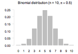
The bar graph displays the probability function of the binomial distribution with n = 10 and π = 0.5. The graph is symmetrical.

If you cannot view or read this graph, select this link to
open a text version.
Curriculum achievement objectives references
Statistical investigation: Levels (4), (5), (6), (7), (8)
Systematic sampling
A method of sampling from a list of the population so that the sample is made up of every kth member on the list, after randomly selecting a starting point from 1 to k.
Example
Consider choosing a systematic sample of 20 members from a population list numbered from 1 to 836.
To find k, divide 836 by 20 to get 41.8.
Rounding gives k = 42.
Randomly select a number from 1 to 42, say 18.
Start at the person numbered 18 and then choose every 42nd member of the list.
The sample is made up of those numbered
18, 60, 102, 144, 186, 228, 270, 312, 354, 396, 438, 480, 522, 564, 606, 648, 690, 732, 774, 816
Sometimes rounding may cause the sample size to be one more or one less than the desired size.
Curriculum achievement objectives references
Statistical investigation: Levels (7), (8)
Last updated March 17, 2022
TOP


