Glossary page R
Random
Relating to a process in which each outcome has a fixed probability of occurring but, on any trial of the process, the actual outcome cannot be predicted.
See: random sample, random sampling, random variable, randomisation, randomness
Curriculum achievement objectives references
Statistical investigation: Levels 6, 7, 8
Randomness
The concept that although each outcome of a process has a fixed probability, the actual outcome of any trial of the process cannot be predicted.
See: random, random sample, random sampling, random variable, randomisation
Curriculum achievement objectives references
Statistical investigation: Levels 6, 7, 8
Random sample
A sample in which all objects or individuals in the population have the same probability of being chosen in the sample.
A random sample can also be a number of independent values from the same theoretical distribution, without involving a real population.
See: simple random sample
Curriculum achievement objectives references
Statistical investigation: Levels 6, 7, (8)
Random sampling
The process of selecting a random sample.
Curriculum achievement objectives references
Statistical investigation: Levels 6, 7, (8)
Random variable
A property that can have different values because there is an element of chance involved in obtaining any value for the property.
A random variable is often represented by an upper case letter, say X.
Example 1
The random selection of an individual from a population is subject to chance. The height of a selected individual will depend on the individual selected and is therefore a random variable. This may be written as: let X represent the height of a randomly selected individual.
Example 2
The random selection of 10 individuals from a population is subject to chance. The number of left-handed people in a sample of 10 individuals will depend on the individuals selected and is therefore a random variable. This may be written as: let X represent the number of left-handed people in a random selection of 10 individuals.
See: continuous random variable, discrete random variable
Curriculum achievement objectives references
Probability: Levels (7), 8
Randomisation
A method in which chance is used to select a sample from a population or to allocate individual units to groups in an experiment.
Randomisation used in sampling
Randomisation forms the basis of many sampling methods, including random sampling, cluster sampling and stratified sampling, because at some stage individual units are selected, using chance, from a group.
See: cluster sampling, random sample, random sampling, simple random sample, stratified sampling
Randomisation used in experiments
In an experiment the use of chance to allocate experimental units to treatment groups is an attempt to make the characteristics of each group very similar to each other so that if each group was given the same treatment the groups should respond in a similar way, on average.
See: experiment, experimental design principles, randomisation test, re-randomisation
Curriculum achievement objectives reference
Statistical investigation: Level 8
Randomisation test
A procedure used to help conclude whether the outcome of an experiment occurred because a treatment is effective or whether the outcome could have occurred purely by chance.
Example
The purpose of an experiment was to see whether giving very young infants specific exercises could lower the age at which the infants start to walk. As part of this experiment 12 very young male infants were randomly allocated to either the exercise group or the control group. The parents of the six infants allocated to the exercise group were instructed to give their infant a programme of specific exercises for 12 minutes each day. The six infants in the control group had no regular exercise programme. The ages, in months, at which these infants first walked without support was recorded and is shown below.
(Source: Zelazo, P. R., Zelazo, N. A., and Kolb, S. (1972). ‘Walking’ in the Newborn. Science, Vol. 176, pp 314-315.)
| Treatment
| Age (months)
| Age (months)
| Age (months)
| Age (months)
| Age (months)
| Age (months)
|
| Exercise
| 9
| 9.5
| 9.75
| 10
| 13
| 9.5
|
| Control
| 11
| 10
| 10
| 11.75
| 10.5
| 15
|
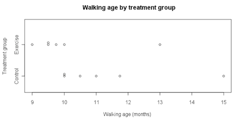
A dot plot of the data is shown below.

If you cannot view or read this diagram/graph, select this link to
open a text version.
In this example we will look at differences in group medians. There is no special reason for choosing to use medians; we could have chosen to look at differences in group means.
Difference in group medians
- = Control group median – Exercise group median
- = 10.750 – 9.625 months
- = 1.125 months
Does the data from the experiment provide any evidence to support the assertion that specific exercises lower the age at which the infants start to walk? In other words, how likely is it that a difference as big as the observed difference of 1.125 months is produced purely by chance?
Would random allocation of the 12 walking ages to the exercise group and the control group often produce a difference in group medians as big as 1.125 months or even bigger? If random allocation alone could easily produce a difference in group medians as big as 1.125 months, or even bigger, then the data from the experiment cannot be interpreted as support that the exercises are effective in lowering the infants’ walking ages. Random allocation to the two groups can be called re-randomisation under chance acting alone.
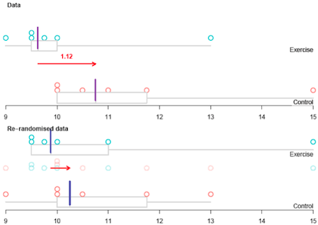
The walking ages from the two groups are combined and six of them are randomly allocated as walking ages for the exercise group, leaving the other six as walking ages for the control group. This is equivalent to assuming there is no link between walking age and treatment group. In other words, the infants would have had the same walking age whether they were in the exercise group or the control group. One such
re-randomisation, produced by the
iNZightVIT software, is shown below.

If you cannot view or read this diagram/graph, select this link to
open a text version.
In this re-randomisation under chance acting alone:
Difference in group medians
- = Control group median – Exercise group median
- = 10.250 – 9.875 months
- = 0.375 months
The ‘randomisation tests’ module from the
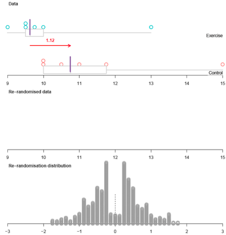
iNZightVIT software carries out 1000 re-randomisations under chance acting alone. The 1000 differences in group medians are plotted in the ‘re-randomisation distribution’ plot in the output below.

If you cannot view or read this diagram/graph, select this link to
open a text version.
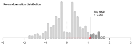
The re-randomisation distribution gives an indication of how likely it is that chance acting alone will produce a difference in group medians as big as 1.125 months or even bigger. Some more output from the ‘randomisation tests’ module is shown below.

If you cannot view or read this diagram/graph, select this link to
open a text version.
Of the 1000 differences in group medians produced by chance acting alone, 58 (5.8%) were as big as, or even bigger than, the observed difference of 1.125 months produced in the experiment itself. This shows that a difference in group medians of 1.125 months or bigger is unlikely to be produced by chance acting alone. Therefore chance probably is not acting alone. We have evidence that chance is not acting alone.
Recall that in the experiment the infants were randomly allocated to the two treatment groups so the characteristics of the two groups (other than the treatment received in the experiment) should be similar to each other. It can be concluded that the data provide evidence that the exercises were effective in lowering the walking age.
At more advanced levels of statistics randomisation tests may be used on data from an observational study.
See: strength of evidence
Curriculum achievement objectives reference
Statistical investigation: Level 8
Randomness
The concept that although each outcome of a process has a fixed probability, the actual outcome of any trial of the process cannot be predicted.
See: random, random sample, random sampling, random variable, randomisation
Curriculum achievement objectives references
Statistical investigation: Levels 6, 7, 8
Range
A measure of spread for a distribution of a numerical variable that is calculated as the difference between the largest and smallest values in the distribution.
The range is less useful than other measures of spread because it is strongly influenced by the presence of just one unusually large or small value; hence the range conveys only one aspect of the spread of the distribution. It is recommended that a graph of the distribution is used to check the appropriateness of the range as a measure of spread and to emphasise its meaning as a feature of the distribution.
Example
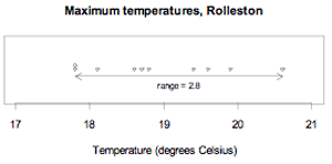
The maximum temperatures, in degrees Celsius (°C), in Rolleston for the first 10 days in November 2008 were: 18.6, 19.9, 20.6, 19.4, 17.8, 18.1, 17.8, 18.7, 19.6, 18.8
The largest value is 20.6°C and the smallest is 17.8°C.
The range of the maximum temperatures over these 10 days is 20.6°C – 17.8°C = 2.8°C
The data and the range are displayed on the dot plot below.

If you cannot view or read this diagram/graph, select this link to
open a text version.
See: measure of spread
Curriculum achievement objectives references
Statistical investigation: Levels (5), (6), (7), (8)
Re-categorising data
The redefining of a variable in some way or the derivation of a new variable from one or more existing variables.
Example 1 (Redefining categories of a category variable)
Consider this question from a questionnaire:
From the given list of types of movies, select the one type that you like best.
Categorising
| Adventure
| □
| Mystery
| □
|
| Comedy
| □
| Romance
| □
|
| Horror
| □
| Science fiction
| □
|
| Martial arts
| □
| Thriller
| □
|
| Melodrama
| □
| Tragedy
| □
|
| Other (please specify): ______________________________________
|
The data could initially be classified into the listed categories. If some categories had a relatively low frequency, then it would be appropriate to re-categorise the data by combining some categories of a similar nature. This is called aggregation. For example, horror, mystery, and thriller could be aggregated to form a ‘suspense’ category. Alternatively, if the ‘Other’ category had a relative high frequency, then the specified responses may suggest some additional categories which could then be used to re-categorise the data.
Example 2 (Expressing the values of a numerical variable in a simpler way)
The values of a variable ‘time’ could initially be recorded as the time from a stopwatch, say 2h 4m 32.4s. For explanation and analysis, all values need to be converted to the time in seconds: 7472.4s for the value above.
Example 3 (Deriving new variables from an existing variable)
From a variable ‘date of birth’ several new variables could be formed, such as ‘age in completed years’, ‘year of birth’, ‘day of birth’, ‘month of birth’, or ‘star sign’.
Example 4 (Deriving a new variable from existing variables)
From the variables ‘height’ and ‘weight’, a new variable ‘body mass index’ can be formed by calculating weight/height2, provided that weight is recorded in kilograms and height is recorded in metres.
Example 5 (Deriving a new variable from existing variables)
From the variables ‘total weekly leisure time’ and ‘weekly time playing sport’, a new variable ‘percentage sport time’ can be formed by weekly time playing sport/total weekly leisure time × 100.
Curriculum achievement objectives references
Statistical investigation: Levels 5, (6), (7), (8)
Regression line
A line that summarises the linear relationship (or linear trend) between the two variables in a linear regression analysis, from the bivariate data collected.
A regression line is an estimate of the line that describes the true, but unknown, linear relationship between the two variables. The equation of the regression line is used to predict (or estimate) the value of the response variable from a given value of the explanatory variable.
Example
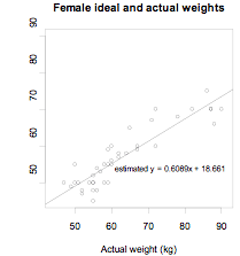
The actual weights and self-perceived ideal weights of a random sample of 40 female students enrolled in an introductory statistics course at the University of Auckland are displayed on the scatter plot below. A regression line has been drawn. The equation of the regression line is predicted y = 0.6089x + 18.661 or predicted ideal weight = 0.6089 × actual weight + 18.661.

If you cannot view or read this graph, select this link to
open a text version.
Alternatives: fitted line, line of best fit, trend line
See: least-squares regression line
Curriculum achievement objectives reference
Statistical investigation: (Level 8)
Relationship
A connection between two variables, usually two numerical variables. Such a connection may not be evident until the data are displayed. A relationship between two variables is said to exist if the connection evident in a data display is so strong that it could not be explained as only due to chance.
Example 1 (Two numerical variables)
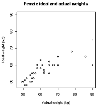
The actual weights and self-perceived ideal weights of a random sample of 40 female students enrolled in an introductory statistics course at the University of Auckland are displayed on the scatter plot below (bottom). In general, as the values of actual weight increase, the values of ideal weight increase. There is clearly a relationship between the variables actual weight and ideal weight.
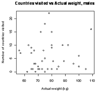
The actual weights and number of countries visited (other than New Zealand) of a random sample of 40 male students enrolled in an introductory statistics course at the University of Auckland are displayed on the scatter plot below (top). There is no clear connection between the variables actual weight and number of countries visited (other than New Zealand).


If you cannot view or read these graphs, select this link to
open a text version.
Example 2 (One numerical variable and one category variable)
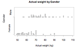
The actual weights of random samples of 40 male and 40 female students enrolled in an introductory statistics course at the University of Auckland are displayed on the dot plot below (bottom). On average, the actual weight of males is greater than that of females. There is clearly a relationship between the variables actual weight and gender.
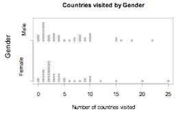
The number of countries visited (other than New Zealand) by random samples of 40 male and 40 female students enrolled in an introductory statistics course at the University of Auckland are displayed on the dot plot below (top). The two sample distributions are quite similar indicating that there is no clear connection between the variables number of countries visited (other than New Zealand) and gender.


If you cannot view or read these graphs, select this link to
open a text version.
Example 3 (Two category variables)
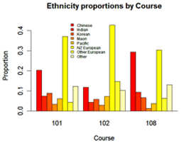
The two sets of bar graphs below display data collected from a random sample of students studying an introductory statistics course at the University of Auckland. They are enrolled in one of three courses: STATS 101, STATS 102, or STATS 108.
The proportions of each ethnic group in each course are displayed on the bar graphs on the left. The three distributions are sufficiently different to indicate that there is a relationship between the variables ethnicity and course.
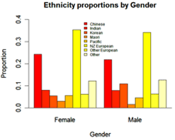
The proportions of each ethnic group for males and females are displayed on the bar graphs on the right. The two distributions are quite similar indicating that there is no clear connection between the variables ethnicity and gender.


If you cannot view or read these graphs, select this link to
open a text version.
See: association
Curriculum achievement objectives references
Statistical investigation: Levels 4, 5, 6, (7), (8)
Relative frequency
For a whole-number variable in a data set, the number of times a value occurs divided by the total number of observations.
For a measurement variable in a data set, the number of occurrences in a class interval divided by the total number of observations.
For a category variable in a data set, the number of occurrences in a category divided by the total number of observations.
In other words, relative frequency = (frequency)/(number of observations)
See: frequency
Curriculum achievement objectives references
Statistical investigation: Levels (4), (5), (6), (7), (8)
Relative risk
The ratio of the risk (or probability) of an event for one group to the risk of the same event for a second group.
Example
The following data were collected on a random sample of students enrolled in a statistics course at the University of Auckland.
Two way table of Course result by Attendance.
|
|
| Attendance
|
|
|
|
| Regular
| Not regular
| Total
|
| Course
| Pass
| 83
| 19
| 102
|
| Result
| Fail
| 17
| 27
| 44
|
|
| Total
| 100
| 46
| 146
|
The risk of failing for students with non-regular attendance = 27/46 = 0.5870
The risk of failing for students with regular attendance = 17/100 = 0.17
The relative risk of failing for students with non-regular attendance compared to those with regular attendance = 0.5870/0.17 = 3.5
This can be interpreted as the risk of failing for students with non-regular attendance is about 3.5 times the risk of failing for students with regular attendance.
Curriculum achievement objectives references
Probability: Levels 7, (8)
Repeated sampling
A process in which samples of the same size are taken repeatedly from the same population.
Curriculum achievement objectives references
Statistical investigation: (Level 8)
Re-randomisation
The process of combining the measurements from two (or more) treatment groups from an experiment and then randomly allocating the measurements from the experimental units to the groups, ensuring the group sizes are the same as they were in the experiment.
This can also be called re-randomisation under chance acting alone. It is important to realise that the experimental units retain their measurements from the experiment when re-randomisation is carried out.
Example
The purpose of an experiment was to see whether giving very young infants specific exercises could lower the age at which the infants start to walk. As part of this experiment 12 very young male infants were randomly allocated to either the exercise group or the control group. The parents of the six infants allocated to the exercise group were instructed to give their infant a programme of specific exercises for 12 minutes each day. The six infants in the control group had no regular exercise programme. The ages, in months, at which these infants first walked without support was recorded and is shown below. (Source: Zelazo, P. R., Zelazo, N. A., and Kolb, S. (1972). ‘Walking’ in the Newborn. Science, Vol. 176, pp 314-315.)
| Treatment
| Age (months)
| Age (months)
| Age (months)
| Age (months)
| Age (months)
| Age (months)
|
| Exercise
| 9
| 9.5
| 9.75
| 10
| 13
| 9.5
|
| Control
| 11
| 10
| 10
| 11.75
| 10.5
| 15
|
One re-randomisation, produced by the
iNZightVIT software, is shown below.

If you cannot view or read this diagram/graph, select this link to
open a text version.
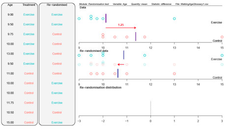
The first panel and the ‘Data’ plot show the data from the experiment. The second panel and the ‘Re-randomised data’ plot show a re-randomisation with random allocation of the walking ages to the two groups (that is, a re-randomisation under chance acting alone).
The arrow on the ‘Data’ plot shows the difference in the group means.
Difference in group means
- = Control group mean – Exercise group mean
- = 1.25 months
The arrow on the ‘Re-randomised data’ plot shows the difference in the group means after re-randomisation.
Difference in group means
- = Control group mean – Exercise group mean
- = -0.25 months
Note: There is no special reason for choosing to use means; we could have chosen to look at differences in group medians.
See: randomisation test, re-randomisation distribution
Curriculum achievement objectives reference
Statistical investigation: Level 8
Re-randomisation distribution
The distribution of a statistic (often a difference in group means or a difference in group medians) calculated from many re-randomisations of the measurements from the experimental units to the treatment groups under chance acting alone.
Example
The purpose of an experiment was to see whether giving very young infants specific exercises could lower the age at which the infants start to walk. As part of this experiment 12 very young male infants were randomly allocated to either the exercise group or the control group. The parents of the six infants allocated to the exercise group were instructed to give their infant a programme of specific exercises for 12 minutes each day. The six infants in the control group had no regular exercise programme. The ages, in months, at which these infants first walked without support was recorded and is shown below. (Source: Zelazo, P. R., Zelazo, N. A., and Kolb, S. (1972). ‘Walking’ in the Newborn. Science, Vol. 176, pp 314-315.)
| Treatment
| Age (months)
| Age (months)
| Age (months)
| Age (months)
| Age (months)
| Age (months)
|
| Exercise
| 9
| 9.5
| 9.75
| 10
| 13
| 9.5
|
| Control
| 11
| 10
| 10
| 11.75
| 10.5
| 15
|
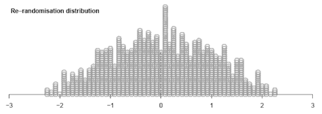
The ‘randomisation tests’ module from the
iNZightVIT software carries out 1000 re-randomisations under chance acting alone. The re-randomisation distribution, showing 1000 differences in group means, is displayed in ‘Re-randomisation distribution’ plot in the output shown below.

If you cannot view or read this diagram/graph, select this link to
open a text version.
Note: There is no special reason for choosing to use means; we could have chosen to look at differences in group medians.
See: randomisation test, re-randomisation
Curriculum achievement objectives reference
Statistical investigation: Level 8
Resample
A sample formed by sampling from an original sample or data set. Bootstrapping is a resampling method used at level 8.
Example
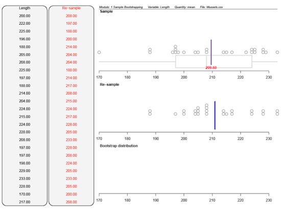
The lengths (in mm) of a sample of 25 horse mussels from a site in the Marlborough Sounds are: 200, 222, 225, 196, 188, 205, 208, 225, 197, 188, 214, 204, 224, 215, 224, 228, 208, 197, 197, 198, 229, 233, 228, 170, 217
The ‘bootstrap confidence intervals’ module from the
iNZightVIT software produced the following output.

If you cannot view or read this diagram/graph, select this link to
open a text version.
The first panel and the ‘Sample’ plot show the original sample. The second panel and the ‘Re-sample’ plot show a resample, using bootstrapping, from the original sample.
Although there was only one value of 200mm in the sample this value occurred twice in the resample. Some values in the sample, such as 170mm and 222mm, did not occur in the resample. The vertical lines on the ‘Sample’ plot and the ‘Re-sample’ plot are the respective means. Means are displayed because the mean (rather than the median) was selected within the software module.
See: bootstrapping
Curriculum achievement objectives references
Statistical investigation: Level 8
Resampling
A process in which samples are taken repeatedly from an existing sample or an existing data set. Bootstrapping is a resampling method used at level 8.
See: bootstrapping
Curriculum achievement objectives references
Statistical investigation: Level 8
Residual (in linear regression)
The difference between an observed value of the response variable and the value of the response variable predicted from the regression line.
From bivariate data to be used for a linear regression analysis, consider one observation, (xi,yi). For this value of the explanatory variable, xi, the value of the response variable predicted from the regression line is
 , giving a point (
 ) that is on the regression line. The residual for the observation (xi,yi) is
 .
.
Example
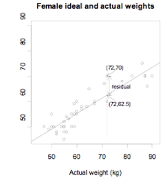
The actual weights and self-perceived ideal weights of a random sample of 40 female university students enrolled in an introductory statistics course at the University of Auckland are displayed on the scatter plot below. A regression line has been drawn. The equation of the regression line is predicted y = 0.6089x + 18.661 or predicted ideal weight = 0.6089 × actual weight + 18.661.
Consider the female whose actual weight is 72 kg and whose self-perceived ideal weight is 70 kg.
Her predicted ideal weight is 0.6089 × 72 + 18.661 = 62.5 kg.
The residual for this observation is 70 kg – 62.5 kg = 7.5 kg.
This is also displayed on the scatter plot.

If you cannot view or read this graph, select this link to
open a text version.
Alternative: prediction error
Curriculum achievement objectives reference
Statistical investigation: (Level 8)
Response variable
The variable, of the two variables in bivariate data, which may be affected by the other variable, the explanatory variable.
If the bivariate data result from an experiment, then the response variable is the one that is observed in response to the experimenter having manipulated or selected the value of the explanatory variable.
In a scatter plot, as part of a linear regression analysis, the response variable is placed on the y-axis (vertical axis).
Alternatives: dependent variable, outcome variable, output variable
Curriculum achievement objectives reference
Statistical investigation: (Level 8)
Risk
An alternative name for probability. The risk of an event occurring is the probability of the event occurring and is mainly used when the event is related to a health issue or is an undesirable event.
Example
The following data were collected on a random sample of students enrolled in a statistics course at the University of Auckland.
Two way table of Course result by Attendance.
|
|
| Attendance
|
|
|
|
| Regular
| Not regular
| Total
|
| Course
| Pass
| 83
| 19
| 102
|
| Result
| Fail
| 17
| 27
| 44
|
|
| Total
| 100
| 46
| 146
|
Based on this sample of students, the risk of failing = 44/146 = 0.30
The risk of failing for students with regular attendance= 17/100 = 0.17
Curriculum achievement objectives references
Probability: Levels 7, (8)
Last updated October 16, 2013
TOP


