Understanding true probability, model estimates, and experimental estimates

Teacher notes

In this discussion we describe three interconnected ways of how we can think about the probability of an event. We can also think in the same three ways about the probabilities of a collection of events or a probability distribution of outcomes but these are not addressed in the discussion.

The model probability or theoretical probability of an event is the probability assigned under a given model. The experimental probability of an event is the probability obtained from trials or simulations, which are based on some underlying assumptions (for example, independence of trials). Both the model probability and the experimental probability of an event give estimates of the “true” probability. Both of these methods for determining the probability of an event are interconnected and they both are seeking to determine the “true” probability of an event, which is usually unknown.

Some illustrations of how we can think about the probability of an event

True probability is the (almost always) unknown actual probability that an event will occur in a given situation.  The actual or “true” probability of a particular coin landing heads up may be affected by the asymmetry of the two faces of the coin, a flaw in its manufacture etc, so may not be exactly 0.5. However, the model (theoretical) probability of a fair coin landing heads of 0.5 could be considered a good model estimate of the “true” probability.  We can also find out about the unknown true probability by observation (experiment) through determining the proportion of heads in a large number of tosses, and using this proportion as an estimate of the “true” probability.

In probability, an experiment is one or more trials of a probability situation. An experimental estimate of an event occurring is calculated from observation as the number of successful trials divided by the total number of trials when the number of trials is sufficiently large.  In the long run (over many trials), the experimental estimate may approach the true probability and may approach the model probability if it can be determined and if it is a good model of the situation (for example, symmetry of a die, or scenario has binomial distribution characteristics).  An experimental estimate that a coin will land heads if it is tossed 20 times and lands heads up 14 times is 14/20 = 0.7.

A probability model is a representation of a situation involving probability. Probability models can incorporate experimental estimates and assumptions about the situation (for example, independence). These assumptions may be based on an idealised view of the world or an understanding of the mathematics of probability, and prior knowledge (for example, recognising the scenario could be modelled by the Poisson distribution). 

A model estimate is an estimate of the probability that an event will occur, based on a probability model. The model estimate of a fair coin landing heads is 0.5. If a probability model is a good representation of the situation, the experimental estimate of an event occurring over many trials will be close to the model estimate. A model must always be considered in context. A good model is one which is fit for the purpose for which it is being used.  When tossing an approximately fair coin, the model estimate of P(heads) = 0.5 is a good model for most purposes. A transportation engineer wishing to set up the timing of traffic lights so that traffic flows smoothly will require a more complex model, tested against experimental observations to ensure that it is fit for the purpose.

In some situations there is no obvious probability or theoretical model, so we can only estimate the probabilities and probability distributions via experiment. These estimates can then be used as a basis for building a probability or theoretical model. For instance, to develop a model of the probability of getting a basketball through the hoop, an initial model might assume a constant probability of 0.5. As data are gathered, there could be successive refinements of the model so that it becomes a better estimate of the true probability. The data might indicate that the probability of getting the ball in the hoop is closer to 0.2 and that it changes over time.

Sometimes we might think that an obvious probability or theoretical model applies, but experimental estimates demonstrate that our model is a poor one. There is now a need to find a better model using the estimates from the experiments. We might initially model the result of spinning a coin as P(heads) = 0.5 but realise that that estimate is a poor one and use data to improve it. The P(heads) = 0.5 idea is based on the assumption that the 2 outcomes are equally likely using the physical symmetry of the coin and prior knowledge about tossing a coin.

Notes:

1. Many books and teachers refer to “the” probability of an event. We need to be clear what is “the” probability we are referring to. Is it the model (theoretical) probability or the experimental probability?
2. When doing probability experiments we need to be clear that we are determining the experimental estimate of the probability of an event not “the” probability of the event.
3. Probability is a difficult philosophical issue and many books have been written about how it could be viewed. The above view is derived from a probability modelling perspective.

Some examples of true probability, model estimates, and experimental estimates

Example 1

What is the probability that the next baby born in New Zealand will be a boy? The true probability that the next baby will be a boy is unknown. There is no theoretical model to base our probability on. 

We can develop an initial model estimate of the probability a baby is a boy, based on our prior knowledge (our hunch). This might be P(boy) = 0.5, or might use knowledge from other sources, so might be P(boy)= 0.525 (international data from Statistics NZ).

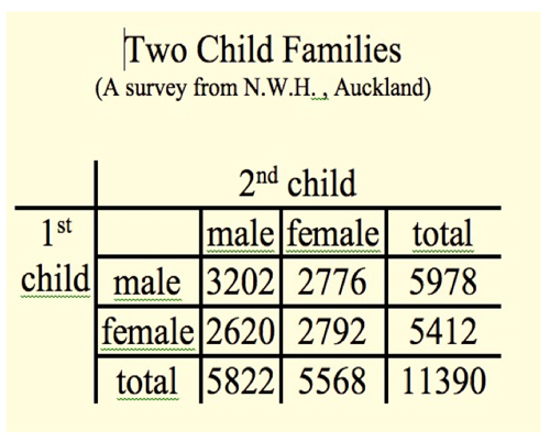
If we can get some experimental data, we can use it to estimate the probability of a baby being a boy, compare this estimate to our initial model probability and develop a better model probability. Experimental data in probability can be any results of observation of the situation. We have some data which was collected from National Women’s hospital in Auckland in the 1990s. Is the data going to be useful? It is old, only from Auckland, and not randomly selected. The data was collected by a hospital, which is likely to be a reliable source of data. The sample was large. The proportion of male children born is unlikely to have changed since the 1990s or to be different in Auckland than in the rest of NZ. We can decide that this data will be useful as the basis of an experimental estimate of the probability of a baby being a boy.

Out of 22 780 births (2 children each from 11 390 families), 11 800 were boys, so our experimental estimate of the probability of the next baby born in NZ being a boy is 11 800/22 780 = 0.5180. These are observations so we need to decide what sort of rounding will be useful for our estimate of probability. Based on a sample of 22 780, we might decide that an experimental estimate of probability to three decimal places is appropriate (SD = root( p (1-p)/N) ≈ 1%).

Our experimental estimate of the probability of the next child in NZ being a boy is 0.518. This is a better model probability to use than our initial model probability based on our hunch, so we change our model estimate of the probability to P(boy) = 0.518. The unknown true probability has not changed, but our model estimate of it is now likely to be closer to the true probability than our initial model probability was. Any new information we get about the probability of a baby being born a boy can be compared to our new model estimate.

Example 2

Two families with two children each live next door to each other. What is the probability that both those families have two boys?  From the National Women’ Hospital data above we can get an experimental estimate of the probability of a two-child family having two boys P(two boys) = 3202/11 390 = 0.2811. Using this experimental data and what we know about theoretical probability, we can create a model for the probability of the distribution of two two-child families. We can assume that people move next door to each other for reasons other than the gender of their children so that the gender of the children can be assumed to be independent of whether the two-child families are next door to each other. Since we are considering two independent random variables, the probability of both families having two boys is 0.2811 × 0.2811 = 0.0790. Our model estimate for the probability of two two-child families both having two boys is 0.08 or about 8% of all pairs of two child families.

Example 3

Is this gamble a good bet? Model estimates of probability can incorporate complex aspects of probability, and may be based on theoretical probability alone. The history of probability includes many examples of model estimates of probability developed by gamblers.

If you throw a pair of dice 24 times, is your probability of getting at least one double six more than 0.5, allowing a gambler to make money in the long run on an even-money bet? Assuming that the gambler uses fair dice, the model estimate based on theoretical probability alone will be a good estimate of the true probability, provided the theoretical model is an accurate representation of the context. The experimental estimate of probability will approach the true probability over the long run. The experimental estimate of probability can be compared with the model estimate to evaluate whether the model is an accurate representation of the context. A gambler playing the same game many times over needs a precise estimate of their probability of winning. A good theoretical model can provide that level of precision, but it is only fit for purpose if it is an accurate representation of the context. The Chevalier de Méré lost money when betting on getting at least one double six in 24 throws of two dice based on his initial model, but later calculated that the probability was 1 – (35/36)²⁴  = 0.4914, and stopped making that losing bet.

Last updated February 21, 2023

TOP