Activity: Lateness – choice or chance
AOs |
Indicators |
Outcomes |
Snapshot |
Learning experiences
Assessment |
Spotlight
Purpose
The purpose of this activity is to demonstrate probability modelling processes that combine data driven and theoretical approaches.
Achievement objective
S8-4 Investigate situations that involve elements of chance:
- C – applying distributions such as the Poisson, binomial, and normal.
Indicators
C. Applying distributions such as the Poisson, binomial, and normal:
They learn that some situations that satisfy certain conditions can be modelled mathematically. The model may be
Poisson,
binomial,
normal, uniform, triangular, or others, or be derived from the situation being investigated.
- Recognises situations in which probability distributions such as
Poisson,
binomial, and
normal are appropriate models, demonstrating understanding of the assumptions that underlie the distributions.
- Selects and uses an appropriate distribution to model a situation in order to solve a problem involving probability.
Specific learning outcomes
Students will be able to:
- select an appropriate theoretical probability distribution model by considering the information provided and the conditions needed to apply the distribution
- use simulations to investigate the effect of sample size on variation
- identify and describe key features of distributions
- identify and discuss “poor” and “good” probability models.
Diagnostic snapshot(s)
Teachers should check for student understanding of random situations before beginning this activity. Students may have formed their own generalisations that any situation that can be represented using proportions, fractions, or percentages can also be considered as a chance event. Students could be given statements like the ones below, and asked to identify whether the process behind the statement is random:
- It is estimated that 15% of NZ drivers speed (drive a car too fast).
- 286 cases of food poisoning were reported last week for a small city of 28,103 people.
- Three fifths of Wellingtonians get their hair cut every four weeks.
- 23.1% of customers waited on hold for more than 5 minutes when they called customer service last week.
It may be helpful to ask students to consider the following when considering these statements:
- How comfortable do you feel asking for the probability of each associated event?
- Is there uncertainty for the event? Are there varied outcomes for the event? Why is there variation? What does uncertainty mean here? If you randomly choose a person then ….
TOP
Planned learning experiences
Provide students with the information below and ask them to discuss the situation and the distribution provided (Note: Percentages or counts have deliberately not been provided for the distribution to keep the focus on the visual features of the distribution.)
Nearly all online stores allow customers to give feedback on their experience by rating the service received. A government organisation monitoring online stores suspects one company is placing fake feedback on their website.
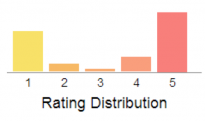
The distribution of ratings for this online store (based on 303 reviews) is shown below:
Note: 1 is the lowest rating and 5 is the highest rating.
Students should be able to identify that the distribution is very clearly bimodal, with most of the ratings on either 1 or 5. Students could estimate the mean rating by considering the height of the bar for each rating and considering this as a weight. By this reasoning, exactly 3 could not be the mean, as the ratings for 4 and 5 combined would be more than the ratings for 1 and 2 combined, and so the mean will be pulled up from 3 towards 4.
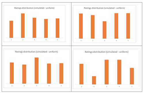
However, we do need to be careful about describing shape and features of distributions (such as bimodality) as these could be caused by chance variation for small data sets. To investigate this with students, simulations can be run to visualise variation in the ratings distribution from chance alone. For example, if we started by assuming a uniform distribution (each rating having a 20% chance of being given), then different simulations (using a spread sheet) could produce different experimental distributions like the ones shown below (based on 303 ratings):

Students should compare the experimental distributions obtained using simulations and decide that the features of the rating distribution (the strong bimodality) are not likely to be caused from chance acting alone with a uniformly distributed random variable.
The strong bimodality of this ratings distribution should prompt discussion related to the suspicion that “the company is placing fake feedback on their website”. Potential issues such as self-selection, where perhaps only customers with really strong opinions about the company have given feedback (for example, based on really good experiences or really bad experiences), could be other explanations for these features.
Introduce the context of students arriving late to class, and lead a discussion around whether students can determine whether they are late to class or not. This could be linked to personal experiences of similar situations of teachers arriving late to class, workers arriving late to their workplace, friends arriving late for coffee and so on.
A scenario like the one below could then be given to students:
A form teacher had an argument with her students regarding lateness to form class over the school year. For this school, form class is at the start of each school day. The teacher argued that arriving late to class is a decision, and that each individual student can determine whether to be late to form class or not. The students argued that arriving late to class is out of their control and that whether they arrive late to form class or not is driven by random processes.
The form teacher accepts that perhaps there may be some chance factors that could cause students to be late and wants to develop a model for lateness to form class so she can determine how many students she could expect to be late to any one form class, and at what number of students would it be very unlikely for only chance to be explaining the lateness.
The teacher’s lateness data shows students in the class were late to 4.5% of the possible form classes (200), and the form class has 30 students.
A completely theoretical modelling approach to this situation could involve selecting an appropriate probability distribution by considering the information provided. For example, the binomial distribution could be selected based on a fixed number of trials (30 students), a fixed probability of success (4.5% probability of being late), and only two outcomes (late or not late). Further assumptions of independence may be made (for example, assuming that one student arriving late is independent from another student in the class arriving late) in order to use this distribution, even if the knowledge students have of this context might suggest this to be an invalid assumption. Using the theoretical distribution, a probability could be calculated (for example, the probability of 5 or more students in a class of 30 arriving late), and the size of this probability used to reach a conclusion.
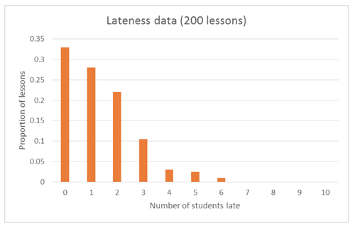
A data driven modelling approach, which also considers theoretical models, could be used to explore the situation. For example, a graph of the actual data collected by the teacher could be shown to students (from the 200 form classes of the year):

Students could be asked to describe the features of this distribution, including how this data shows that “students have been late to 4.5% of form classes”. For example, they may describe the general shape as “positively skewed” or “triangular” (although this is a discrete distribution), and estimate the mean of the distribution to be somewhere between 1.2 – 1.5 students (which is around 4.5% of 30 students). Depending on their prior knowledge and experience working with binomially distributed random variables, they may be able to discuss that they would expect the proportions/counts to be the highest around the mean for the distribution, and this does not appear to be happening with this data.
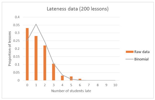
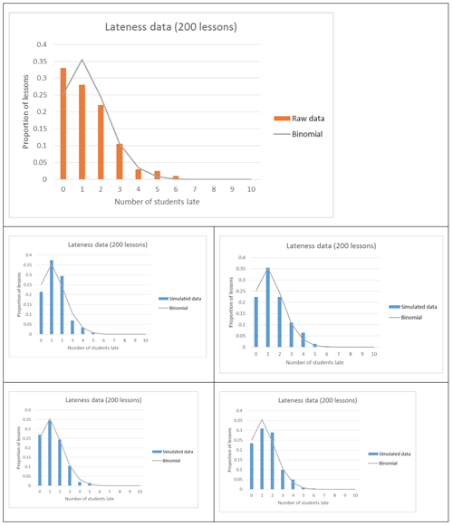
A binomial model can be fitted to the data to allow students to compare the theoretical binomial distribution (with n = 30 and p = 0.045) with the data collected by the teacher:

Students should be able to identify that the shapes of the distributions do not match between the theoretical and raw data, in particular the theoretical model peaks on “one student”, whereas the raw data peaks on “no students”. Since we have raw data, there will be some error or chance variation, and so students should expect not to see a perfect fit between the raw and theoretical model. However, they also need to have an appreciation for how much data they have, and how this may increase the size of the variation, for example, is the theoretical model a poor fit because it does not model the situation well, or does it look like a poor model because we do not have enough data to see clearly what is happening?
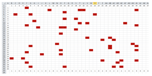
Students can set up a “roll book” for a class of 30 students and 200 form classes, and carry out simulations to see the variation in proportions for the numbers of students late:

In this example, each cell contains the formulae =IF(RANDBETWEEN(1,1000)<=45,"L","")
The last row uses a COUNTIF function to find the total number of students late for each lesson (form class). A spreadsheet file is available.
Students should run the simulations many times, and compare the features of the distributions they get from the simulated data and the features of the theoretical distribution. Examples of simulated distributions, compared to raw data:

Students should be able to identify that while the theoretical model and simulated data (for 200 lessons) do not match perfectly, the mode of “no students” from the raw data is not occurring in the simulated data, so it does not appear that the binomial model (with n = 30 and p = 0.045) is a good model, even when taking into account the variation expected from having data from only 200 lessons.
At this point, there should be some discussion with students around why the theoretical model (binomial n = 30, p = 0.045) appears to be a poor model for lateness to this form class. If the assumption is accepted that lateness is a random process, could there be some days where there might be a higher chance of lateness than others? Students should be able to identify factors such as weather, traffic accidents, major events, road works, Mondays being the first day back after the weekend as related variables that might influence the percentage of students arriving late to form class.
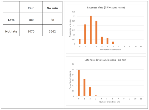
Students can then be given a two way table for the data, which categorises the number of late lessons by days on which there was rain or not, as well as the lateness data presented earlier split into days on which there was rain or not.

Students can be asked “Based on this data, are students more likely to be late to form class on days where there is rain compared to days where there is no rain?”
Visually, the distributions of number of students late for days where there is rain and days where there is no rain have different centres and shapes.
Using the two way table, 8% of students were late on days with rain, compared to 2.2% of students on days without rain.
Reviewing this new information about the lateness data should prompt students to consider using two models for lateness: one for rainy days and one for other days. The binomial distribution could be used as a theoretical model, but with different values for p for the two types of days (see below):

Students should compare the raw data with the theoretical models and feel happy with deeming these to be “good models”. While the fit is “looser” for the rain days, students should be able to explain that this may be because there is only data for 75 lessons, so they would expect this.
Now that the students have “good models”, they should be able to identify that on rainy days, 6 or more students arriving late would be unlikely, but on non-rainy days, 3 or more students arriving late would be unlikely, assuming lateness is a random process.
Returning to the notion that lateness is a choice and not a chance event, students should also consider the data from a “student perspective”. In applying the binomial distribution as the theoretical model, assumptions need to be made concerning randomness and independence. How confident are the students (based on their personal experience of this situation) that we can assume that the 4.5% used as the probability of lateness can be applied to all students? This can be reworded as a “4.5% chance of any student arriving late to any form class”. While we have looked at a factor that might influence which form classes may have more lateness than others, students need to look at the data based on “lessons late by student” to further investigation notions of independence.
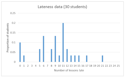
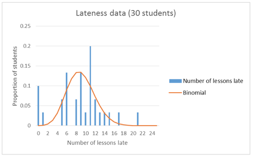
The graph below can be given to students, which shows the distribution of number of lessons (form classes) late for the class of 30 students:

Students should be asked to describe the key features of this distribution (centre, spread, shape, unusual features), and make a link between the 4.5% and the mean (which can be estimated from the graph to be somewhere between 9 – 10 lessons). This distribution does not appear to have a clear shape, and links should be made back to the fact this is only data for 30 students (the one form class).
The raw data could be compared to a theoretical model (binomial distribution with n = 200 and p = 0.045):

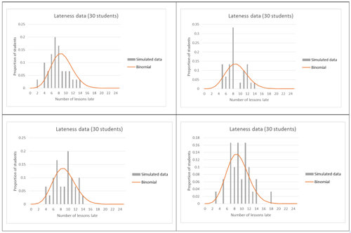
Students should be able to identify that while the theoretical model with these parameters should look fairly symmetrical and even approximately normal, the raw data is very “choppy” and has high proportions at the lowest and highest values (number of lessons late). Again, reference should be made to the fact that this is only data for 30 students, so this lack of fit may not be a model issue, but a lack of data issue. To investigate this, students can run simulations (similar to those run for the number of students late per lesson), and compare this simulated data to the theoretical model:

Students should be able to identify that while the theoretical model and simulated data (for 30 students) do not match perfectly, getting 0, 1 or 21 lessons late is not occurring in the simulated data. So these features of the raw data do not appear to be a product of chance variation and a small amount of data. A discussion can then happen with the students around whether this could be considered as evidence that there is “choice” involved in whether a student is late to form class or not.
The activity should finish by asking students to reflect on the modelling process, and whether, now having found “good models” for lateness to this form class, these models would remain fixed in the future. They should consider whether the percentage of students arriving late to form class might change over time, whether interventions by the form class teacher may have an impact, and other events such as students leaving or joining the form class.
Possible adaptations to the activity
- Spinners could be used for learning to use tables and tree diagrams to solve probability problems.
TOP
Planned assessment
This teaching and learning activity could lead towards assessment in the following achievement standards:
Spotlight on
Pedagogy
Planning for effective learning
Planning should involve:
- starting with familiar contexts, concrete materials and prior knowledge, and moving to generalisations and abstract ideas (and back and forth between these as needed).
Encouraging reflective thought and action
Examples of teacher actions that encourage reflective thought and action for students:
- Supporting students to explain and articulate their thinking.
- Encouraging students to fine-tune their statistical thinking.
Key competencies
Using language, symbols and texts
- Students use statistical language to pose questions and communicate findings.
- Students interpret and communicate mathematical and statistical information and ideas, they know and use specialised vocabulary, as well as their own language, to explain ideas.
Managing self
- Students develop skills of independent learning.
- Students are prepared to take risks, make decisions, and persevere.
- Students are self-motivated, resilient, know their own strengths and weaknesses, and have a ‘can-do’ attitude.
- Students set goals, rise to new challenges, ask for help if needed, and take ownership of their learning.
- Students plan and manage time effectively.
Values
- Students will be encouraged to value:
- innovation, inquiry, and curiosity, by thinking critically, creatively, and reflectively
- ecological sustainability, which includes care for the environment.
Māori/Pasifika
Planning for content and language learning
Last updated September 17, 2018
TOP


