How to find the shortest path
Trial and error |
Benefits of an algorithm |
Example: Method 1 |
Dijkstra’s algorithm
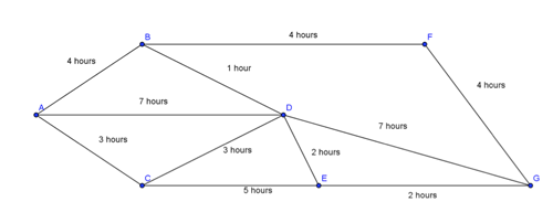
This network shows the tramping tracks in a regional park in Northland. The weights of the edges are the times in hours that it will take to tramp each track. These times are written on the DOC signposts at track junctions.
Ana is planning a tramp from A to G and wants to do the tramp in the shortest time. What tracks should she take?

Tramping tracks
Trial and error
Teachers can encourage students to find their own way of solving this problem. Many are likely to develop an algorithm as they do this.
This network is relatively simple. It’s not difficult to find the shortest path by trial and error. You could list all the paths from A to G, then choose the one with the smallest weight. (See the route inspection problem number 3 in the traversability notes for an example.)
A common trial and error method is to branch out from the starting vertex along paths until you reach the vertex you require, keeping track of the distance travelled from the starting point. You can also remove paths as you go if you find a shorter one.
This is is all very well for small graphs, with few vertices, but not so good for large graphs as it quickly becomes too cumbersome to keep track of what you are doing.
TOP
Benefits of using an algorithm
If you want to show your thinking as you solve this problem, then an algorithm (step procedure) is useful.
Another advantage of using an algorithm is that it can be written as a computer program to solve more complicated problems. For example, airlines use an algorithm to solve problems like this when planning their schedules for international flights.
TOP
Example: Method one
We now show a method of doing this that a student might use, and then a generally known method, Dijkstra’s Algorithm.
Notation: Let w(e) be the weight of edge e. For example, in the graph above w(AC) =3.
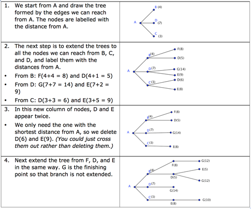
The algorithm is displayed as a tree while we work through the process.

Tramping tracks

Method 1 - tree

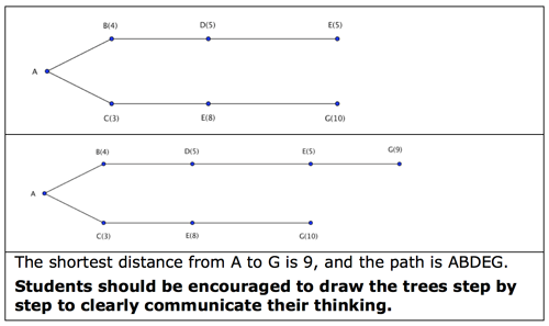
Method 1 - shortest distance
Note: This method is using a kind of “branch and bound” technique to search the graph. At each stage, it branches out to all the vertices reached from the previous vertices. It then prunes or removes vertices as it goes, if the numbers or bounds on the vertices are too large. This is a commonly used technique widely employed by computer scientists, with many advantages and disadvantages.
TOP
Dijkstra’s algorithm
The idea is to start out with one vertex and branch out by selecting new vertices until we reach the vertex we want or until all vertices are reached.
The vertices are divided into three groups:
- those already confirmed
- those being considered as adjacent to one of the confirmed vertices
- those not yet seen.
Each step looks at the vertices that can be reached from the previous steps.
Every vertex considered gets a temporary label, which is the shortest distance so far of the vertex from the starting point.
As different routes are discovered, and all but the shortest route to the end of each step are discarded, a vertex is confirmed, and its temporary label is replaced by a permanent one.
Step 1
Start with one vertex, and give it a permanent label of zero. This vertex is now a confirmed vertex.
Step 2
- Take the most recently confirmed vertex u with permanent label of d, say.
- Look at each vertex v adjacent to u that has not yet got a permanent label.
- If v has no label, then give it a temporary label of d+w(uv).
- If the sum of d and the weight of the edge uv (d+w(uv)) is less than the temporary label of v, then change the temporary label of v to this smaller value.
Step 3
- Look at all the vertices with temporary labels.
- Choose the vertex w with the smallest temporary label. (If there are several of equal value, select whichever you prefer.)
- Make this label permanent and change w into a confirmed vertex.
Step 4
- Repeat the last two steps until all vertices are confirmed.
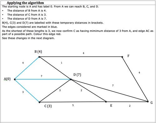
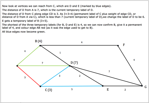
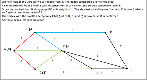
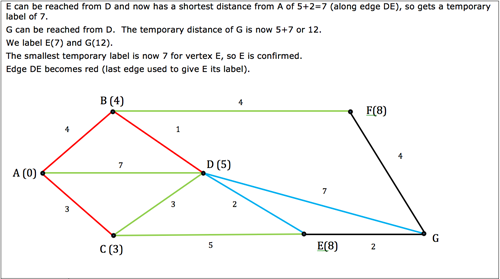
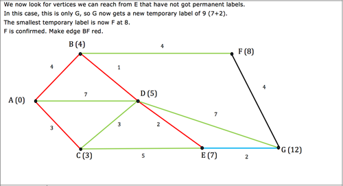
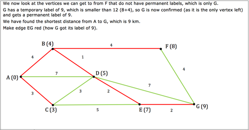
Look through the following example to see how the algorithm works. We colour the edges used as we go.

Dijkstra’s Algorithm_step 4
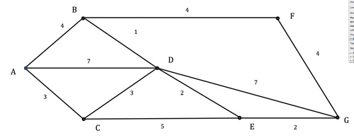
The original diagram

Original diagram - part1

Original diagram - part2

Original diagram - part3

Original diagram - part4

Original diagram - part5

Original diagram - part6

Original diagram - part7
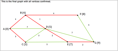
To find the shortest route, we work backwards from G, and choose the length of the edge which is equal to the difference in the labels.
The labels for G and E are 9 and 7, and the length of the edge GE is 2. This is on the shortest path.
Note that the difference of the labels for the nodes on all other edges from G is not equal to the distance of the edge, so we do not use them. For example G(9) and F(8) 9–8 = 1 but FG = 4.
From E: The labels for E and D are 7 and 5 and ED=2. This is on the shortest path. (E(7) and C(3) is another alternative, but 7–3=4 and the path CE is 5).
From D: The labels for D and B are 5 and 4 and DB=1. This is on the shortest path.
From B we can go straight to A.
Retracing these edges we find the shortest path is ABDEG and its length is 9.
Students should be encouraged to redraw the network and indicate the labelling and edges considered at each step in the algorithm to clearly communicate their thinking.
Notes:
- As we were going along, we were colouring edges red when confirming vertices chosen. This was to help illustrate how the algorithm works. It was where the difference between the labels of the new confirmed vertex and an already confirmed adjacent vertex equalled the weight of the edge used. This was not mentioned in the earlier description of the algorithm above, but was done in the example. So basically we go back from G to A along red edges to find the shortest route.
- G happens to be the last vertex found. We have also found the shortest path to all vertices in the graph from A.
- You can now go back and see that method one pretty much also follows this algorithm. In fact, in step 3, you may have noticed that in the top branch D had a label of 5, while in the middle D had a label of 7. This means that the middle branch could then have been removed.
- It is possible to have a network with two or more shortest paths of the same length. The path that is chosen will then depend on decisions made whilst constructing the path.
Things to ponder
Students might like to think about and explore:
- What happens if two or more vertices have the same smallest temporary label?
- What if you want the shortest distance from A from G? D from A? D from B? D from C? D from G?
Students can use whichever display for following Djikstra’s algorithm they wish.
< back to AO M7-5
Last updated May 1, 2012
TOP


