Glossary page C
Category data
Data in which the values can be organised into distinct groups. These distinct groups (or categories) must be chosen so that they do not overlap and that every value belongs to one and only one group, and there should be no doubt as to which one.
The term ‘category data’ is used with two different meanings. The curriculum uses a meaning that puts no restriction on whether or not the categories have a natural ordering. This use of category data has the same meaning as qualitative data. The other meaning restricts category data to categories that do not have a natural ordering.
Example
The eye colours of a class of year 9 students.
Alternative: categorical data
See: qualitative data
Curriculum achievement objectives references
Statistical investigation: Levels 1, 2, 3, 4, (5), (6), (7), (8)
Category variable
A property that may have different values for different individuals and for which these values can be organised into distinct groups. These distinct groups (or categories) must be chosen so that they do not overlap and that every value belongs to one and only one group, and there should be no doubt as to which one.
The term ‘category variable’ is used with two different meanings. The curriculum uses a meaning that puts no restriction on whether or not the categories have a natural ordering. This use of category variable has the same meaning as qualitative variable. The other meaning of category variable is restricted to categories which do not have a natural ordering.
Example
The eye colours of a class of year 9 students.
Alternative: categorical variable
See: qualitative variable
Curriculum achievement objectives references
Statistical investigation: Levels (4), (5), (6), (7), (8)
Causal-relationship claim
A statement that asserts that changes in a phenomenon (the response) are caused by differences in a received treatment or by differences in the value of another variable (an explanatory variable).
Such claims can be justified only if the observed phenomenon is a response from a well-designed and well-conducted experiment.
Curriculum achievement objectives reference
Statistical literacy: Level 8
Census
A study that attempts to measure every unit in a population.
Curriculum achievement objectives references
Statistical literacy: Levels (7), (8)
Central limit theorem
The fact that the sampling distribution of the sample mean of a numerical variable becomes closer to the normal distribution as the sample size increases. The sample means are from random samples from some population.
This result applies regardless of the shape of the population distribution of the numerical variable.
‘Central’ is used in this term because there is a tendency for values of the sample mean to be closer to the ‘centre’ of the population distribution than individual values are. This tendency strengthens as the sample size increases.
‘Limit’ is used in this term because the closeness or approximation to the normal distribution improves as the sample size increases.
See: sampling distribution
Curriculum achievement objectives reference
Statistical investigation: Level 8
Centred moving average
See: moving mean
Curriculum achievement objectives reference
Statistical investigation: (Level 8)
Chance
A concept that applies to situations that have a number of possible outcomes, none of which is certain to occur when a trial of the situation is performed.
Two examples of situations that involve elements of chance follow.
Example 1
A person will be selected and their eye colour recorded.
Example 2
Two dice will be rolled and the numbers on each die recorded.
Curriculum achievement objectives references
Probability: All levels
Class interval
One of the non-overlapping intervals into which the range of values of measurement data, and occasionally whole-number data, is divided. Each value in the distribution must be able to be classified into exactly one of these intervals.
Example 1 (Measurement data)
The number of hours of sunshine per week in Grey Lynn, Auckland, from Monday 2 January 2006 to Sunday 31 December 2006 are recorded in the frequency table below. The class intervals used to group the values of weekly hours of sunshine are listed in the first column of the table.
Hours of sunshine frequency table, by 5 hour class intervals.
| 5 to less than 10
| 2
|
| 10 to less than 15
| 2
|
| 15 to less than 20
| 5
|
| 20 to less than 25
| 9
|
| 25 to less than 30
| 12
|
| 30 to less than 35
| 10
|
| 35 to less than 40
| 5
|
| 40 to less than 45
| 6
|
| 45 to less than 50
| 1
|
| Total
| 52
|
Example 2 (Whole-number data)
Students enrolled in an introductory statistics course at the University of Auckland were asked to complete an online questionnaire. One of the questions asked them to enter the number of countries they had visited, other than New Zealand. The class intervals used to group the values are listed in the first column of the table.
Number of countries visited frequency table, by 4 country class intervals.
| 0 – 4
| 446
|
| 5 – 9
| 172
|
| 10 – 14
| 69
|
| 15 – 19
| 19
|
| 20 – 24
| 14
|
| 25 – 29
| 4
|
| 30 – 34
| 3
|
| Total
| 727
|
Alternatives: bin, class
Curriculum achievement objectives references
Statistical investigation: Levels (4), (5), (6), (7), (8)
Cleaning data
The process of finding and correcting (or removing) errors in a data set in order to improve its quality.
Mistakes in data can arise in many ways, such as:
- A respondent may interpret a question in a different way from that intended by the writer of the question.
- An experimenter may misread a measuring instrument.
- A data entry person may mistype a value.
Curriculum achievement objectives references
Statistical investigation: Levels 5, (6), (7), (8)
Cluster (in a distribution of a numerical variable)
A distinct grouping of neighbouring values in a distribution of a numerical variable that occur noticeably more often than values on each side of these neighbouring values. If a distribution has two or more clusters, then they will be separated by places where values are spread thinly or are absent.
In distributions with a small number of values or with values that are spread thinly, some values may appear to form small clusters. Such groupings may be due to natural variation (see sources of variation), and these groupings may not be apparent if the distribution had more values. Be cautious about commenting on small groupings in such distributions.
For the use of ‘cluster’ in cluster sampling see the description of cluster sampling.
Example 1
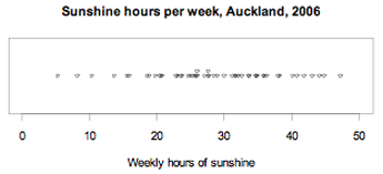
The number of hours of sunshine per week in Grey Lynn, Auckland, from Monday 2 January 2006 to Sunday 31 December 2006 are displayed in the dot plot below.

If you cannot view or read this graph, select this link to
open a text version.
From the greater density of the dots in the plot, we can see that the values have one cluster from about 23 to 37 hours per week of sunshine.
Example 2
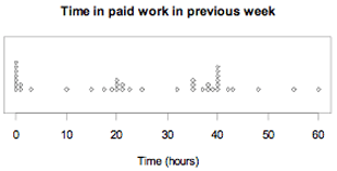
A sample of 40 parents was asked about the time they spent in paid work in the previous week. Their responses are displayed in the dot plot below.

If you cannot view or read this graph, select this link to
open a text version.
There are three clusters in the distribution: a group who did a very small amount or no paid work, a group who did part-time work (about 20 hours) and a group who did full-time work (about 35 to 40 hours).
Curriculum achievement objectives references
Statistical investigation: Levels (2), (3), (4), (5), (6)
Statistical literacy: Levels (2), (3), (4), (5), (6)
Cluster sampling
A method of sampling in which the population is split into naturally forming groups (the clusters), with the groups having similar characteristics that are known for the whole population. A simple random sample of clusters is selected. Either the individuals in these clusters form the sample or simple random samples chosen from each selected cluster form the sample.
Example
Consider obtaining a sample of secondary school students from Wellington. The secondary schools in Wellington are suitable clusters. A simple random sample of these schools is selected. Either all students from the selected schools form the sample or simple random samples chosen from each selected school form the sample.
Curriculum achievement objectives references
Statistical investigation: Levels (7), (8)
Coefficient of determination (in linear regression)
The proportion of the variation in the response variable that is explained by the regression model.
If there is a perfect linear relationship between the explanatory variable and the response variable, there will be some variation in the values of the response variable because of the variation that exists in the values of the explanatory variable. In any real data, there will be more variation in the values of the response variable than the variation that would be explained by a perfect linear relationship. The total variation in the values of the response variable can be regarded as being made up of variation explained by the linear regression model and unexplained variation. The coefficient of determination is the proportion of the explained variation relative to the total variation.
If the points are close to a straight line, then the unexplained variation will be a small proportion of the total variation in the values of the response variable. This means that the closer the coefficient of determination is to 1, the stronger the linear relationship.
The coefficient of determination is also used in more advanced forms of regression, and is usually represented by R2. In linear regression, the coefficient of determination, R2, is equal to the square of the correlation coefficient, i.e., R2 = r2.
Example
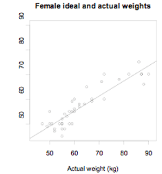
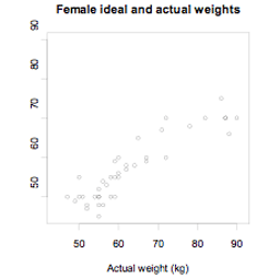
The actual weights and self-perceived ideal weights of a random sample of 40 female students enrolled in an introductory statistics course at the University of Auckland are displayed on the scatter plot below. A regression line has been drawn. The equation of the regression line is
predicted y = 0.6089x + 18.661 or predicted ideal weight = 0.6089 × actual weight + 18.661

If you cannot view or read this graph, select this link to
open a text version.
The coefficient of determination R2 = 0.822
This means that 82.2% of the variation in the ideal weights is explained by the regression model (i.e., by the equation of the regression line).
Curriculum achievement objectives reference
Statistical investigation: (Level 8)
Combined event
An event that consists of the occurrence of two or more events.
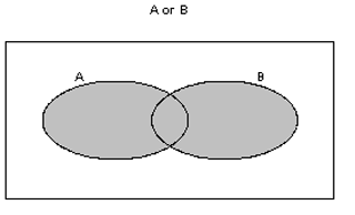
Two different ways of combining events A and B are: A or B, A and B.
A or B is the event consisting of outcomes that are either in A or B or both.

If you cannot view or read this diagram, select this link to
open a text version.
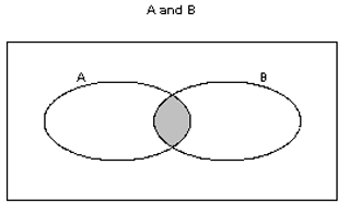
A and B is the event consisting of outcomes that are common to both A and B.

If you cannot view or read this diagram, select this link to
open a text version.
Example
Suppose we have a group of men and women and each person is a possible outcome of a probability activity. A is the event that a person is a woman and B is the event that a person is taller than 170cm.
Consider A and B. The outcomes in the combined event A and B will consist of the women who are taller than 170cm.
Consider A or B. The outcomes in the combined event A or B will consist of all of the women as well as the men taller than 170cm. An alternative description is that the combined event A or B will consist of all people taller than 170cm as well as the women who are not taller than 170cm.
Alternative: compound event, joint event
Curriculum achievement objectives reference
Probability: Level 8
Complementary event
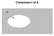
With reference to a given event, the event that the given event does not occur. In other words, the complementary event to an event A is the event consisting of all of the possible outcomes that are not in event A.
There are several symbols for the complement of event A. The most common are A' and Ā.

If you cannot view or read this diagram, select this link to
open a text version.
Example
Suppose we have a group of men and women and each person is a possible outcome of a probability activity. If A is the event that a person is aged 30 years or more, then the complement of event A, A', consists of the people aged less than 30 years.
Curriculum achievement objectives reference
Probability: (Level 8)
Conditional event
An event that consists of the occurrence of one event based on the knowledge that another event has already occurred.
The conditional event consisting of event A occurring, knowing that event B has already occurred, is written as A | B, and is expressed as ‘event A given event B’. Event B is considered to be the ‘condition’ in the conditional event A | B.
The probability of the conditional event A | B, P(A|B) = P(A and B)/P(B) .
For a justification of the above formula, see the example below.
Example
Suppose we have a group of men and women and each person is a possible outcome of the probability activity of selecting a person. A is the event that a person is a woman, and B is the event that a person is taller than 170cm.
Consider A | B.
Given that B has occurred, the outcomes of interest are now restricted to those taller than 170cm.
A | B will then be the women of those taller than 170cm.
Suppose that the genders and heights of the people were as displayed in the two-way table below.
Two-way table of Height by Gender.
|
|
| Height
|
|
|
|
| Taller than 170cm
| Not taller than 170cm
| Total
|
| Gender
| Male
| 68
| 15
| 83
|
| Female
| 28
| 89
| 117
|
|
| Total
| 96
| 104
| 200
|
Given that B has occurred, the outcomes of interest are the 96 people taller than 170cm.
If a person is randomly selected from these 96 people, then the probability that the person is female is P(A|B) = 28/96 = 0.292.
If both parts of the fraction are divided by 200, this becomes P(A|B) = (28/200)/(96/200) = P(A and B)/P(B)
Curriculum achievement objectives reference
Probability: Level 8
Confidence interval
An interval estimate of a population parameter. A confidence interval is therefore an interval of values, calculated from a random sample taken from the population, of which any number in the interval is a possible value for a population parameter.
The word ‘confidence’ is used in the term because the method that produces the confidence interval has a specified success rate (confidence level) for the percentage of times such intervals contain the true value of the population parameter in the long run. 95% is commonly used as the confidence level.
See: bootstrap confidence interval, bootstrapping, margin of error
Curriculum achievement objectives reference
Statistical investigation: Level 8
Confidence level
A specified percentage success rate for a method that produces a confidence interval, meaning that the method has this rate for the percentage of times such intervals contain the true value of the population parameter in the long run.
The most commonly used confidence level is 95%.
The confidence level associated with the process of forming a bootstrap confidence interval for a parameter cannot be determined accurately but, in most cases, the confidence level will be about 90% or higher (especially if any samples used are quite large). That is, just because the central 95% of estimates was used to form the bootstrap confidence interval we cannot say that the confidence level is 95%.
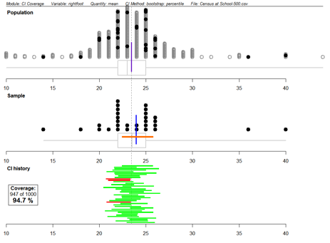
This confidence level concept can be illustrated using the ‘Confidence interval coverage’ module from the
iNZightVIT software. The module produced the following output. Note that to use this module you must have data on every unit in the population.

If you cannot view or read this diagram/graph, select this link to
open a text version.
The population used is 500 students from the CensusAtSchool database. This is multivariate data. The variable ‘rightfoot’ (the length of a student’s right foot, in centimetres), the quantity ‘mean’, the confidence interval method ‘bootstrap: percentile’, the sample size ‘30’ and the number of repetitions ‘1000’ were selected.
The ‘Population’ plot shows the population distribution of the right foot lengths of the 500 students in the population. The vertical line shows the true population mean (about 23.4cm). The darker dots show the final random sample selected.
The true population mean is also shown as a dotted line through all three plots.
The ‘Sample’ plot shows the 30 foot lengths from the sample, the sample mean (vertical line) and the bootstrap confidence interval (horizontal line).
The ‘CI history’ plot shows bootstrap confidence intervals constructed from some of the samples. The bootstrap confidence intervals that contained (covered) the true population mean are shaded in a light colour (green) and the bootstrap confidence intervals that did not contain (did not cover) the true population mean are shaded in a dark colour (red). The box gives the percentage success rate of the bootstrap confidence interval process based on 1000 samples. The success rate of 94.7% estimates the confidence level when using the bootstrap confidence interval process on this population and for this sample size.
Alternative: coverage
See: bootstrap confidence interval, bootstrapping
Curriculum achievement objectives reference
Statistical investigation: (Level 8)
Confidence limits
The lower and upper boundaries of a confidence interval.
Curriculum achievement objectives reference
Statistical investigation: (Level 8)
Continuous distribution
The variation in the values of a variable that can take any value in an (appropriately-sized) interval of numbers.
A continuous distribution may be an experimental distribution, a sample distribution, a population distribution, or a theoretical probability distribution of a measurement variable. Although the recorded values in an experimental or sample distribution may be rounded, the distribution is usually still regarded as being continuous.
Example
At Levels 7 and 8, the normal distribution is an example of a continuous theoretical probability distribution.
See: distribution
Curriculum achievement objectives references
Statistical investigation: Levels (5), (6), (7), (8)
Probability: Levels (5), (6), 7, (8)
Continuous random variable
A random variable that can take any value in an (appropriately-sized) interval of numbers.
Example
The height of a randomly selected individual from a population.
Curriculum achievement objectives references
Probability: Levels (7), 8
Correlation
The strength and direction of the relationship between two numerical variables.
In assessing the correlation between two numerical variables, one variable does not need to be regarded as the explanatory variable and the other as the response variable, as is necessary in linear regression.
Two numerical variables have positive correlation if the values of one variable tend to increase as the values of the other variable increase.
Two numerical variables have negative correlation if the values of one variable tend to decrease as the values of the other variable increase.
Correlation is often measured by a correlation coefficient, the most common of which measures the strength and direction of the linear relationship between two numerical variables. In this linear case, correlation describes how close points on a scatter plot are to lying on a straight line.
See: correlation coefficient
Curriculum achievement objectives reference
Statistical investigation: Level (8)
Correlation coefficient
A number between -1 and 1 calculated so that the number represents the strength and direction of the linear relationship between two numerical variables.
A correlation coefficient of 1 indicates a perfect linear relationship with positive slope. A correlation coefficient of -1 indicates a perfect linear relationship with negative slope.
The most widely used correlation coefficient is called Pearson’s (product-moment) correlation coefficient, and it is usually represented by r.
Some other properties of the correlation coefficient, r:
- The closer the value of r is to 1 or -1, the stronger the linear relationship.
- r has no units.
- r is unchanged if the axes on which the variables are plotted are reversed.
- If the units of one, or both, of the variables are changed, then r is unchanged.
Example
The actual weights and self-perceived ideal weights of a random sample of 40 female students enrolled in an introductory statistics course at the University of Auckland are displayed on the scatter plot below.

If you cannot view or read this graph, select this link to
open a text version.
The correlation coefficient r = 0.906
See: coefficient of determination (in linear regression), correlation
Curriculum achievement objectives reference
Statistical investigation: (Level 8)
Cyclical component (for time-series data)
Long-term variations in time-series data that repeat in a reasonably systematic way over time. The cyclical component can often be represented by a wave-shaped curve, which represents alternating periods of expansion and contraction. The successive waves of the curve may have different periods.
Cyclical components are difficult to analyse, and at Level 8 cyclical components can be described along with the trend.
See: time-series data
Curriculum achievement objectives reference
Statistical investigation: (Level 8)
Last updated September 27, 2013
TOP


